Part 8 of From Saturday to Co-Author. Part 7 covered the charge decomposition. This series is dedicated to Stephen Jordan.
Everything in this series so far has been infrastructure. The fold, the gradient, the cost algebra, the test harness, the charge decomposition, the manual adjoint. This post is about a single number that all of it was for: the expected satisfaction fraction $\tilde c$ of exact finite-depth QAOA at depth fourteen on regular MaxCut, computed on a Mac.
The phase of the project this post covers, in the timeline of Part 1, is the MaxCut follow-on (Phase 2), which began the day after the XORSAT paper was submitted on 27 April. It is the second half of the “two stories” the series is telling: the same engine, the same algebra, the same test harness, a different problem family, eight weeks later.
The arithmetic of $p = 14$
The charge evaluator from Part 7 is $O(p \cdot 4^p)$. Forward cost roughly quadruples for each unit of $p$ added. The manual charge adjoint is roughly $4.5 \times$ forward, independent of $p$. By the standards of where the project started, that is enormously generous: $p = 14$ should take about eight or nine hours of wall clock on a workstation. The wall clock is not the constraint.
The constraint is memory.
Each level of the charge evaluator caches a per-channel tensor of $4^p$ complex doubles. At $p = 14$, that is $4^{14}$ entries times sixteen bytes, roughly 4.3 GB per level. The instrumented forward (which retains those tensors so the backward can read them) holds them for all $p$ levels simultaneously, with additional ping-pong buffers and coefficient adjoint state. The naive accounting on the working set at $p = 14$ projected somewhere around 122 GB.
The Mac Studio has 64 GB.
There were two responses to this. The dishonest one was to run the result on a bigger machine and quietly omit the Mac from the headline. The honest one was to write a sequence of memory fixes that brought the working set inside 64 GB, and let the Mac compute the actual production number. The latter took most of a week.
Five fixes, in two buckets
The fixes split cleanly into two strategies. The first three trade work for memory; the last two trade memory for work.
Time for space: drop intermediate state on the forward, recompute it during the backward.
-
_bwd_root!originally retained a full history of root-state tensorsfhistfor the backward to consume. This was the single largest peak contributor, on the order of 60 GB at $p = 14$. The fix removedfhistentirely; the backward replays the relevant forward step on demand. The cost is a near-doubling of the work along the root-backward path. The saving is most of the peak. -
_bwd_branch!Phase 1 retained a similar historyp1sof about 13 GB. The fix replaces it with two ping-pong buffers and a replay from the seed. Same trade, smaller scale. -
charge_expectation_and_gradientoriginally let the cache linger across the whole call. The fix drops consumed entries eagerly: as soon ascache.children[lv],cache.states[lv]andcache.F_levels[lv-1]are no longer needed, they are released. The freed memory shows up immediately rather than at the end of the function.
Space for time: precompute and alias to avoid extra allocations.
-
The
_bwd_root!buffer strategy was cleaned up:w_finalis precomputed once instead of recomputed in the loop; the large temporaries are hoisted outside the loop; the factor adjoints share an explicit ping-pong pair instead of allocating fresh ones. -
_charge_branch_instrumentedincludes an $m = 1$ alias optimisation: when the multiplicity is one, the post-power tensor is the same object as the input, andt_normalizedaliasesF_poweredrather than copying. One full vector per level saved.
Net effect: the working set at $p = 14, D = 3$ comes in at 55.65 GB peak resident. The Mac Studio handles it. At $D = 4$ the peak is 56.51 GB. At $D = 5$ it is stable around 56 GB while the optimiser still runs.
The fixes are commodity engineering. None of them is mathematically clever. They are the kind of work that takes a careful diff, a careful benchmark before, and a careful benchmark after, and that is invisible in any paper but is the difference between “we ran this on a cluster” and “we ran this on a workstation.” The code is in src/charge_manual_adjoint.jl on branch feature/charge-adjoint-memory-fix, commit 74cf598, for anyone who wants to compare diffs.
The diagnostics module
An earlier $p = 14$ attempt, before the memory fixes landed, was killed silently by the operating system overnight. The Julia process disappeared. The terminal was at a shell prompt in the morning. No stack trace, no message, no recovery file; just a system log entry saying the kernel had reclaimed the process for memory pressure.
That class of failure is not a bug in any individual line of code. It is the absence of infrastructure that should report what the code is doing in time for the report to outlive the process. The next morning the project gained one of its unglamorous load-bearing pieces, the Diagnostics module.
The design that survived:
- Environment-controlled, off by default.
QAOA_DIAG=1turns it on;QAOA_DIAG=2adds per-iteration memory snapshots. No code changes to enable or disable. - Zero-cost when disabled. The diagnostic checks compile down to a
Ref{Bool}branch the optimiser predicts away. The overhead when off is indistinguishable from no diagnostics at all on benchmarks. - Phase-tagged. Every long-running entry point (
forward,cache,backward_root,backward_phase2,backward_phase1,optimiser_step) is wrapped in a phase marker. The current phase is always known. - Atexit hook. A finaliser registered with
atexitwrites the last known phase, the last completed iteration, the current best $\tilde c$, and the current angles to a recovery file. The hook fires even when the process is being torn down by a signal; the hook itself is wrapped intry/catchbecause writing to stderr during process exit is allowed to fail and we do not want that failure to mask the original one. - Memory tracking.
Sys.maxrss()is recorded at every phase boundary. A growing high-water mark across iterations is the signature of a leak; a flat high-water mark with a sudden jump at a specific iteration is the signature of OOM. Either way, the log has the evidence.
The module is unexciting. It is also why the second $p = 14$ run, with the memory fixes installed and diagnostics enabled, produced a result rather than another silent corpse.
The numbers
The Phase 2 results to date, all on the Mac Studio M4 (64 GB unified memory, Julia 1.12.5), all for regular MaxCut ($k = 2$):
k=2, D=3, p=14:  c̃ = 0.891384992947   wall = 32 343 s  (8.98 h)   peak RSS = 55.65 GB
k=2, D=4, p=14:  c̃ = 0.831514625400   wall = 18 958 s  (5.27 h)   peak RSS = 56.51 GB
k=2, D=5, p=14:  c̃ = 0.801254018370   wall = 22 501 s  (6.25 h)   peak RSS = 56.39 GB
k=2, D=6, p=14:  c̃ = 0.771627233507   wall = 17 859 s  (4.96 h)   peak RSS = 54.95 GB
k=2, D=7, p=14:  c̃ = 0.752436836526   wall = 20 852 s  (5.79 h)   peak RSS = 55.05 GB
k=2, D=8, p=14:  c̃ = 0.735341340823   wall = 14 489 s  (4.02 h)   peak RSS = 56.50 GB
k=2, D=9, p=14:  c̃ = 0.721906666140   wall = 17 512 s  (4.86 h)   peak RSS = 52.53 GB
Those are exact expected satisfaction fractions of depth-fourteen QAOA on infinite-graph $D$-regular MaxCut, computed by an exact evaluator with a hand-derived manual adjoint, on a single workstation. The seven $p = 14$ rows together account for about forty hours of wall clock on a machine that fits under a desk. Eight hours and fifty-nine minutes of that is the $D = 3$ run.
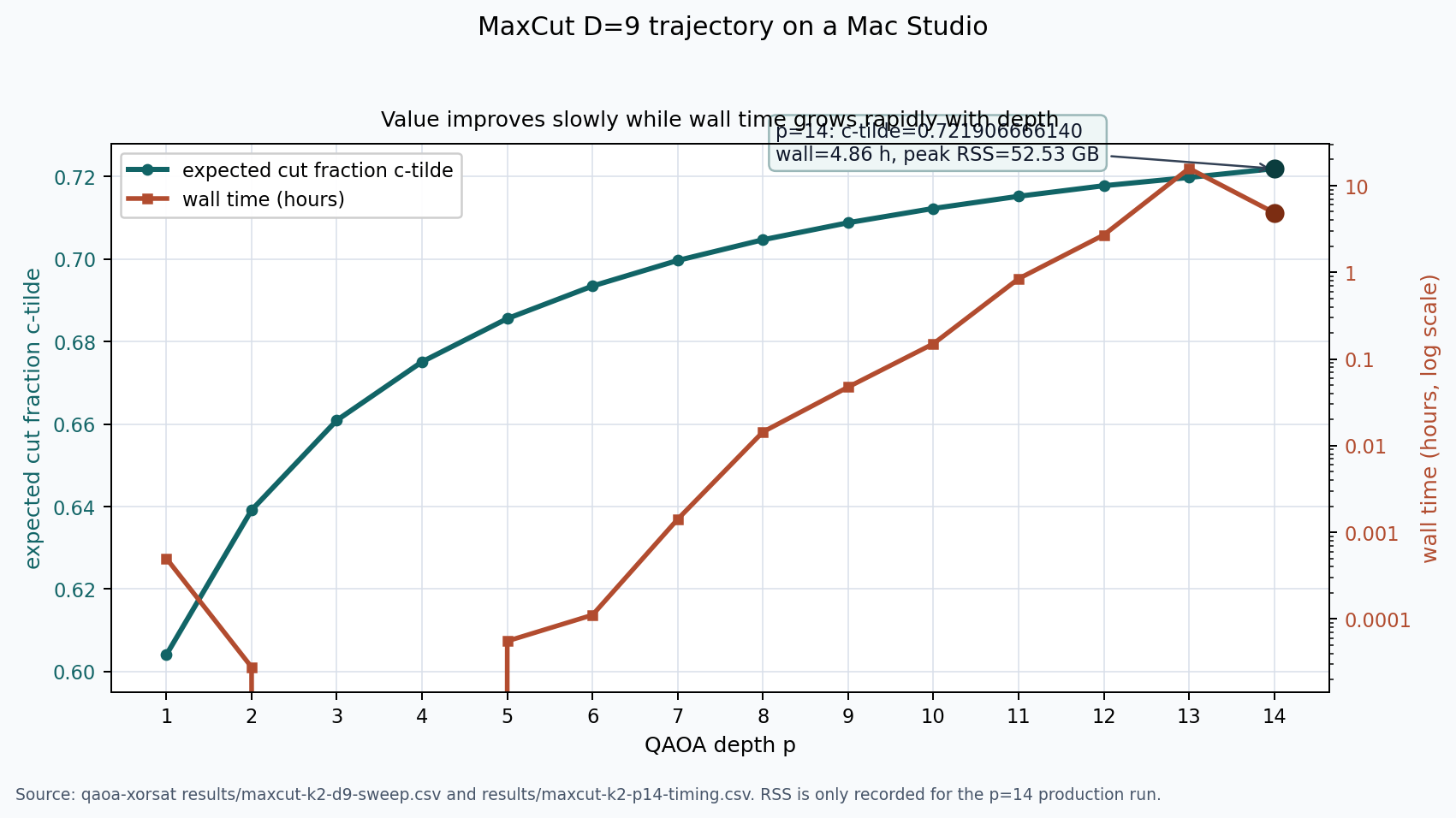
The $D = 9$ trajectory shows the shape of the tradeoff. The value improves steadily but by smaller increments as $p$ grows, while wall time moves onto a log scale. Peak RSS is only recorded for the final $p = 14$ production run, so the memory number appears as an annotation rather than a false memory-vs-depth curve. The $p = 13$ and $p = 14$ wall times come from different production runs, so the wall-time curve should be read as observed runtime, not a smooth scaling fit.
What this beats and by how much
The relevant classical benchmarks for $D$-regular MaxCut are tight. Comparison is worth making because comparison is what the field was waiting for.
- Goemans–Williamson SDP worst case on any MaxCut instance: $\tilde c \geq 0.8786$.
- DQI (Decoded Quantum Interferometry) explicit upper bound for $D$-regular MaxCut: $\tfrac{1}{2} + \tfrac{1}{2\sqrt{D - 1}}$. At $D = 3$ this is $0.854$; at $D = 7$ it is $0.704$.
- Infinite-depth QAOA ceiling for 3-regular MaxCut, from local-tree analysis: $\tilde c_\infty \approx 0.9326$.
Across the seven $p = 14$ rows, the QAOA value clears the DQI explicit bound at every $D$, by between 0.038 ($D = 3$) and 0.051 ($D = 5$). At $D = 3$, the value of $0.891384992947$ additionally clears the Goemans–Williamson worst-case guarantee by about 0.013 and sits below the infinite-depth 3-regular ceiling by about 0.041.
These are the precise statements. They are narrow. $D$-regular MaxCut on the infinite-graph limit is a stylised setting; the Goemans–Williamson bound is a worst-case guarantee that holds on any graph, which is a stronger property than the expectation-value claim of QAOA on a regular family. The comparison the field has been waiting for is the one where exact numbers can be put side by side, because exactness is what stops both sides from over-claiming. The fact that the QAOA value beats the strongest classical lower bound on this family at every $D$ we ran, by an amount that exceeds the numerical uncertainty in either, is the comparison.
What I am not claiming
The discipline of Part 1 is the discipline I want to keep here.
I am not claiming “QAOA beats classical algorithms.” I am claiming “exact finite-depth QAOA at $p = 14$ on infinite-graph $D$-regular MaxCut clears the DQI explicit upper bound at every $D \in {3, 4, 5, 6, 7, 8, 9}$, and additionally clears the Goemans–Williamson worst-case guarantee at $D = 3$.” That sentence has every qualifier it needs.
I am not claiming that $p = 14$ on a Mac is a computational miracle. It is not. It is the consequence of three independent factor-of-$p$-class speedups stacked: the WHT factorisation from Part 2, the charge decomposition from Part 7, and the manual adjoint from Part 3 and its charge variant. Each of those was a small piece of mathematics; the headline number is what happens when they compose.
I am not claiming that the diagnostics module is interesting. It is profoundly uninteresting. It is the boring infrastructure without which $p = 14$ on commodity hardware would have remained a half-hour of compute, an empty log, and a missing process. The number above the table is the result; the diagnostics module is what makes the number trustworthy enough to put in a table.
What the project demonstrates, narrowly:
- The depth ceiling that previously required cluster compute and GPU acceleration is reachable on a Mac, across multiple values of regularity, with the right algorithmic stack.
- The infrastructure is open. The code, the tests, the diagnostics, the memory-fix diffs, and the result files are public. Anyone who wants to reproduce $p = 14$ at any $D \in {3, 4, 5, 6, 7, 8, 9}$ can do so on the same kind of hardware.
- The same engine that produced these numbers is the engine that produced the Phase 1 paper’s fifteen-instance XORSAT sweep. One fold, two problem families, three precision regimes, four gradient strategies, two phases of the project, the same compiled code. That is the algebra from Part 5 doing what it was for.
Everything in this post was built in conversation. Some of the conversations were with Stephen. Some were with the JPM team’s published code in QOKit. Some were with an AI coding assistant whose role in this project has been substantial and continuous from day two; the next post unpacks the disciplines that made working with that assistant productive.
Next: The collaborator that never sleeps, on the disciplines and techniques that made eight weeks of AI-assisted research productive, and the shape of the human contribution alongside an instrument that can produce a tested module in twenty minutes.
Code: github.com/johnazariah/qaoa-xorsat. The five memory fixes are on branch feature/charge-adjoint-memory-fix, commit 74cf598, in src/charge_manual_adjoint.jl. The diagnostics module is src/diagnostics.jl. The $p = 14$ result summary is results/maxcut-k2-p14-timing.csv; the individual $D = 8$ and $D = 9$ traces are under results/maxcut-k2-d{8,9}-p14-*.