How to Raise e to a Matrix (and Why You'd Want To)

A first-principles account of why \(\lvert\psi(t)\rangle = e^{-iHt}\lvert\psi_0\rangle\) solves the Schrödinger equation, and what that formula means geometrically. The whole story is carried by one running example, the \(2\times2\) Hermitian matrix \(H=\begin{pmatrix}2&1\\1&2\end{pmatrix}\).

0. Orientation: what we are building toward

The time-dependent Schrödinger equation (with \(\hbar=1\)) is the first-order linear ODE

\[\dot{\psi} = -iH\psi,\qquad \psi(0)=\psi_0,\]

where \(H\) is a Hermitian operator (the Hamiltonian). The claim to be understood is that its solution is

\[\lvert\psi(t)\rangle = e^{-iHt}\lvert\psi_0\rangle.\]

Two questions have to be answered to make this meaningful and then intuitive:

1. What does it mean to exponentiate a matrix, and why does the result solve the ODE?
2. Why is \(e^{-iHt}\) a rotation of state space (so probability is conserved), and what is actually rotating?

The path runs: scalar exponential, matrix exponential, the Hermitian hypothesis, spectral decomposition (the "shadow" picture), two bases, functions of \(H\), the propagator as rotation, the geometry of phase, interference, and finally the connection to machine learning through a single factor of \(i\).

---

1. The matrix exponential, and why it solves the ODE

1.1 Start from the scalar case

For one number \(a\), the ODE \(\dot{x}=ax\), \(x(0)=x_0\) has the solution

\[x(t)=e^{at}x_0,\qquad e^{at}=\sum_{k=0}^{\infty}\frac{(at)^k}{k!}.\]

That series is the Taylor (Maclaurin) expansion of \(e^x\) at \(x=at\). Recall the general Taylor expansion about \(0\),

\[f(x)=\sum_{k=0}^{\infty}\frac{f^{(k)}(0)}{k!}x^k,\]

and note that for \(f(x)=e^x\) every derivative is \(e^x\), so \(f^{(k)}(0)=1\) and

\[e^x=\sum_{k=0}^{\infty}\frac{x^k}{k!}.\]

1.2 Promote the series to matrices

We define the exponential of a square matrix \(M\) by reusing the very same series with \(M\) substituted for \(x\):

\[e^{M}:=\sum_{k=0}^{\infty}\frac{M^k}{k!}.\]

This converges for every finite matrix \(M\), so it is always well-defined. Everything in the series is legal for matrices: \(M^k\) is repeated matrix multiplication, division by \(k!\) is scalar scaling, and the terms are added.

Aside: is this "analytic continuation"? It has the right shape: a formula proven for scalars is reused to define the object in a larger setting, so the power-series coefficients \(1/k!\) are the real content and \(x\) is "whatever you are allowed to plug in." But it is not analytic continuation in the technical sense. Analytic continuation stays inside \(\mathbb{C}\) and is unique (the identity theorem), extending a function to more of the same space where the original series may fail to converge. The matrix exponential instead (i) changes the space, moving from scalars to the noncommutative algebra of \(n\times n\) matrices, and (ii) always converges, so there is no radius to escape and nothing to continue past. The precise name for "give meaning to \(f(M)\)" is functional calculus. Its holomorphic flavor, \(f(M)=\frac{1}{2\pi i}\oint f(z)(zI-M)^{-1}\,dz\), is the genuinely continuation-flavored one; the spectral flavor of Section 5 only needs \(f\) evaluated at the eigenvalues.

1.3 Why \(e^{-iHt}\) solves the ODE

Set \(U(t):=e^{-iHt}=\sum_{k\ge0}\frac{(-iHt)^k}{k!}\) and \(\psi(t):=U(t)\psi_0\). Differentiate term by term (valid because the series converges nicely):

\[\frac{d}{dt}U(t)=\sum_{k\ge1}\frac{(-iH)^k t^{k-1}}{(k-1)!}=(-iH)\sum_{k\ge1}\frac{(-iHt)^{k-1}}{(k-1)!}=(-iH)\,U(t).\]

Therefore \(\dot{\psi}=(-iH)U(t)\psi_0=-iH\psi\), and since \(U(0)=e^0=I\) we get \(\psi(0)=\psi_0\). The formula is exactly the solution.

The rest of this document explains why the exponential is computable and what it means, which is where the Hermitian structure of \(H\) enters.

---

2. The Hermitian hypothesis

Everything below rests on one property of \(H\), so it deserves to come first.

2.1 Definition

A matrix is Hermitian if it equals its own conjugate transpose:

\[H=H^\dagger,\qquad H^\dagger:=\overline{H}^{\,T}.\]

For real matrices, conjugation does nothing, so Hermitian just means symmetric (\(H=H^T\)). Mentally: Hermitian is the complex version of symmetric. Examples: \(\begin{pmatrix}2&1\\1&2\end{pmatrix}\) (real symmetric) and \(\begin{pmatrix}0&-i\\i&0\end{pmatrix}\) (transpose swaps the off-diagonals, conjugation flips their signs back).

2.2 The meaning behind the formula

The content of \(H=H^\dagger\) is a statement about the inner product. The adjoint \(H^\dagger\) is defined by \(\langle a\vert Hb\rangle=\langle H^\dagger a\vert b\rangle\) for all \(a,b\). So Hermitian means

\[\boxed{\ \langle a\vert Hb\rangle=\langle Ha\vert b\rangle\quad\text{for all }a,b.\ }\]

In words: \(H\) can be slid from the right vector to the left vector, and nothing changes. Such an operator is self-adjoint. That single symmetry is the engine for the two facts we need.

2.3 The spectral theorem's three gifts

If \(H\) is Hermitian, then:

1. all eigenvalues \(E_n\) are real;
2. eigenvectors of distinct eigenvalues are orthogonal;
3. there is a complete orthonormal eigenbasis \(\{\lvert n\rangle\}\), with \(\sum_n\lvert n\rangle\langle n\rvert=I\).

The first two fall straight out of the boxed sliding property.

Real eigenvalues. Take \(H\lvert n\rangle=E_n\lvert n\rangle\) with \(\lvert n\rangle\ne0\). Then

\[E_n\langle n\vert n\rangle=\langle n\vert H\vert n\rangle=\langle Hn\vert n\rangle=\overline{E_n}\langle n\vert n\rangle.\]

Since \(\langle n\vert n\rangle=\lVert n\rVert^2>0\), we get \(E_n=\overline{E_n}\): real.

Orthogonality. With \(H\lvert n\rangle=E_n\lvert n\rangle\) and \(H\lvert m\rangle=E_m\lvert m\rangle\),

\[E_n\langle m\vert n\rangle=\langle m\vert H\vert n\rangle=\langle Hm\vert n\rangle=E_m\langle m\vert n\rangle\]

(using \(E_m\) real). So \((E_n-E_m)\langle m\vert n\rangle=0\), and distinct eigenvalues force \(\langle m\vert n\rangle=0\).

2.4 Geometric intuition: pure stretch, no twist

A general matrix can shear, rotate, and have skewed or complex eigenvectors. Two failure modes make the point:

• \(\begin{pmatrix}0&-1\\1&0\end{pmatrix}\) is a \(90^\circ\) rotation; its eigenvalues are \(\pm i\) (complex) and it has no real eigenvectors.
• \(\begin{pmatrix}1&1\\0&1\end{pmatrix}\) is a shear; it has only one eigendirection, is defective, and is not diagonalizable.

A Hermitian matrix is forbidden from either: self-adjointness forces its action to be "choose mutually perpendicular axes and scale along each by a real number." That clean "orthogonal axes plus real scale factors" structure is exactly the spectral decomposition of Section 3. The shadow picture is valid only because \(H\) is Hermitian.

2.5 Hermitian is the generator of unitary

Here is the relationship that ties this to the propagator. The map

\[H\ (\text{Hermitian})\ \longmapsto\ U=e^{-iH}\ (\text{unitary})\]

is the operator version of the scalar fact \(x\ (\text{real})\mapsto e^{ix}\ (\text{on the unit circle})\). Real numbers generate the unit circle; Hermitian operators generate the unitaries (the rotations). The reason is the spectral story: \(H\) Hermitian has real eigenvalues on an orthonormal basis, so \(e^{-iH}\) has the same orthonormal eigenbasis but eigenvalues \(e^{-iE_n}\), which are pure phases (modulus 1) precisely because the \(E_n\) are real. Same orthonormal basis plus all eigenvalues of modulus 1 equals a rotation, that is, a unitary. Hermitian is the steering-wheel angle; unitary is the resulting turn.

---

3. Spectral decomposition and projectors: the shadow picture

This section is the heart. Everything rests on the idea that a projector casts a shadow.

3.1 A projector casts a shadow

Picture a vector \(\lvert\psi\rangle\) in the plane and a single direction, say the \(x\)-axis. The projection of \(\lvert\psi\rangle\) onto that axis is its shadow: drop a perpendicular, keep the \(x\)-part, discard the rest. A projector is the operator that performs that shadow-casting. Two facts about shadows, which become the two key algebraic properties:

• Shadow of a shadow is the same shadow. Projecting twice onto the same axis changes nothing the second time. (This becomes idempotency, \(P^2=P\).)
• Shadows onto perpendicular axes vanish. The shadow onto the \(x\)-axis, then projected onto the \(y\)-axis, is zero. (This becomes orthogonality, \(P_nP_m=0\) for \(n\ne m\).)

3.2 Writing a projector: the outer product

Take a unit vector \(\lvert n\rangle\). Two products:

• Inner product \(\langle n\vert\psi\rangle\): a number, "how much of \(\lvert\psi\rangle\) points along \(\lvert n\rangle\)," the length of the shadow.
• Outer product \(\lvert n\rangle\langle n\rvert\): an operator, the machine that produces the shadow as a vector.

Watch it act:

\[P_n\lvert\psi\rangle=\big(\lvert n\rangle\langle n\rvert\big)\lvert\psi\rangle=\lvert n\rangle\underbrace{\langle n\vert\psi\rangle}_{\text{a number}}=\underbrace{\langle n\vert\psi\rangle}_{\text{how much}}\ \underbrace{\lvert n\rangle}_{\text{which direction}}.\]

Read right to left: measure how much of \(\lvert\psi\rangle\) lies along \(\lvert n\rangle\), then lay that amount down in the direction \(\lvert n\rangle\). Concretely, with \(\lvert0\rangle=(1,0)^T\),

\[P_0=\lvert0\rangle\langle0\rvert=\begin{pmatrix}1&0\\0&0\end{pmatrix},\qquad P_0\begin{pmatrix}a\\b\end{pmatrix}=\begin{pmatrix}a\\0\end{pmatrix}.\]

It keeps the \(x\)-part and zeroes the \(y\)-part: the shadow onto the \(x\)-axis.

3.3 The two magic properties as algebra

Idempotent (shadow of a shadow):

\[P_n^2=\lvert n\rangle\underbrace{\langle n\vert n\rangle}_{=1}\langle n\rvert=\lvert n\rangle\langle n\rvert=P_n.\]

Orthogonal (perpendicular directions ignore each other):

\[P_nP_m=\lvert n\rangle\underbrace{\langle n\vert m\rangle}_{=\,\delta_{nm}}\langle m\rvert.\]

Both at once:

\[\boxed{\ P_nP_m=\delta_{nm}P_n.\ }\]

This is what makes all cross-terms vanish later.

3.4 Completeness: shadows rebuild the vector

For an orthonormal basis, casting shadows onto every direction and adding them rebuilds the original vector:

\[\sum_n P_n=\sum_n\lvert n\rangle\langle n\rvert=I\qquad(\text{resolution of the identity}).\]

Apply it to any \(\lvert\psi\rangle\):

\[\lvert\psi\rangle=I\lvert\psi\rangle=\sum_n\lvert n\rangle\langle n\vert\psi\rangle=\sum_n c_n\lvert n\rangle,\qquad c_n=\langle n\vert\psi\rangle.\]

Every vector is the sum of its components along the basis directions. Completeness says the basis is big enough to see all of \(\lvert\psi\rangle\).

3.5 Spectral decomposition

For Hermitian \(H\),

\[H=\sum_n E_n P_n=\sum_n E_n\lvert n\rangle\langle n\rvert.\]

Intuition: \(H\) is a to-do list. For each eigendirection \(\lvert n\rangle\) it says "multiply by the real number \(E_n\)." To apply \(H\) to any vector: break it into shadows, scale each shadow by its eigenvalue, add them back:

\[H\lvert\psi\rangle=\sum_n E_n c_n\lvert n\rangle.\]

\(H\) does not mix directions; it stretches each eigendirection independently. Check on a basis vector: \(H\lvert m\rangle=\sum_n E_n\lvert n\rangle\langle n\vert m\rangle=E_m\lvert m\rangle\).

3.6 The running example, verified by hand

Use the rotated (diagonal) directions

\[\lvert+\rangle=\tfrac1{\sqrt2}\begin{pmatrix}1\\1\end{pmatrix},\qquad\lvert-\rangle=\tfrac1{\sqrt2}\begin{pmatrix}1\\-1\end{pmatrix}.\]

They are unit length and orthogonal (\(\langle+\vert-\rangle=0\)). Their projectors:

\[P_+=\tfrac12\begin{pmatrix}1&1\\1&1\end{pmatrix},\qquad P_-=\tfrac12\begin{pmatrix}1&-1\\-1&1\end{pmatrix}.\]

Completeness: \(P_++P_-=I\). Orthogonality: \(P_+P_-=0\). Now build a Hermitian matrix by choosing eigenvalues \(E_+=3\), \(E_-=1\):

\[H=3P_++1P_-=\begin{pmatrix}2&1\\1&2\end{pmatrix}.\]

The innocent matrix \(\begin{pmatrix}2&1\\1&2\end{pmatrix}\) is secretly "stretch the \(\lvert+\rangle\) diagonal by 3, stretch the \(\lvert-\rangle\) diagonal by 1." Direct check: \(\begin{pmatrix}2&1\\1&2\end{pmatrix}\begin{pmatrix}1\\1\end{pmatrix}=\begin{pmatrix}3\\3\end{pmatrix}=3\begin{pmatrix}1\\1\end{pmatrix}\).

3.7 Shadow summary

A projector \(P_n=\lvert n\rangle\langle n\rvert\) casts the shadow of a vector onto one direction: measure the amount \(\langle n\vert\psi\rangle\), lay it down along \(\lvert n\rangle\). Shadows onto an orthonormal basis satisfy \(P_nP_m=\delta_{nm}P_n\) (a shadow of itself is itself; perpendicular shadows vanish) and \(\sum_n P_n=I\) (the shadows rebuild the vector). Spectral decomposition \(H=\sum_n E_n P_n\) then says \(H\) is nothing but "stretch each eigendirection by its eigenvalue," which is exactly why functions of \(H\) will be easy.

---

4. Two bases: eigenbasis versus site basis

4.1 A basis is any orthonormal spanning set

Coordinates are basis-relative: the same physical vector has different coordinate-numbers in different bases, and there are infinitely many choices of basis. Two of them are singled out for different reasons.

4.2 The eigenbasis (chosen by \(H\))

The eigenbasis \(\{\lvert+\rangle,\lvert-\rangle\}\) is the set of directions \(H\) only stretches. Its defining feature: \(H\) is diagonal in it,

\[H\ \xrightarrow{\ \text{eigenbasis}\ }\ \begin{pmatrix}3&0\\0&1\end{pmatrix}.\]

Diagonal means no coupling; each direction evolves on its own. This basis is chosen by the operator.

4.3 The site basis (chosen by the physical setup)

The site basis (also called the computational, standard, position, or measurement basis) is a different distinguished basis:

\[\lvert0\rangle=\begin{pmatrix}1\\0\end{pmatrix},\qquad\lvert1\rangle=\begin{pmatrix}0\\1\end{pmatrix}.\]

It is not chosen by \(H\) but by the problem: the labels that carry physical meaning. The name "site" reads \(\lvert0\rangle\) as "the excitation sits on site 0" and \(\lvert1\rangle\) as "site 1"; think of two atoms or two wells side by side. This is where the initial condition and the measurement live.

4.4 \(H\) is not diagonal in the site basis

Written in the site basis, the same operator is

\[H\ \xrightarrow{\ \text{site basis}\ }\ \begin{pmatrix}2&1\\1&2\end{pmatrix}.\]

The diagonal entries (\(2,2\)) are the on-site energies; the off-diagonal entry (\(1\)) is the hopping amplitude, the term that lets the excitation tunnel from site 0 to site 1. That off-diagonal is why the dynamics is nontrivial. The matrix of an operator depends on the basis you write it in: diagonal (\(\mathrm{diag}(3,1)\)) in the eigenbasis, not diagonal in the site basis.

4.5 The two bases are related by a rotation

The eigenvectors in site coordinates, \(\lvert+\rangle=\tfrac1{\sqrt2}(1,1)^T\) and \(\lvert-\rangle=\tfrac1{\sqrt2}(1,-1)^T\), encode a \(45^\circ\) rotation. So the state \(\lvert\psi_0\rangle=\lvert0\rangle\) has site coordinates \((1,0)\), "definitely on site 0," but eigen coordinates \(\left(\tfrac1{\sqrt2},\tfrac1{\sqrt2}\right)\), "an equal superposition of the two energy eigenstates." One vector, two descriptions.

4.6 The method in one line

\[\text{site basis (question)}\ \xrightarrow{\ \text{change}\ }\ \text{eigenbasis (evolve as phases)}\ \xrightarrow{\ \text{change back}\ }\ \text{site basis (read answer)}.\]

The eigenbasis is where time evolution is easy (diagonal, just phases); the site basis is where the physics is posed. The sloshing and interference of later sections exist precisely because these two bases are misaligned. If they coincided, the eigenstates would be the sites, nothing would hop, and there would be no dynamics. Physically, the eigenstates \(\lvert+\rangle\) (energy 3) and \(\lvert-\rangle\) (energy 1) are the delocalized (bonding and antibonding) orbitals spread over both sites; localized-on-a-site is not the same as definite-energy, and that mismatch is the site-versus-eigenbasis distinction made physical.

---

5. Functions of \(H\), and the propagator

5.1 The lever

Because the projectors do not interfere, powers of \(H\) are trivial:

\[H^2=\Big(\sum_n E_nP_n\Big)\Big(\sum_m E_mP_m\Big)=\sum_{n,m}E_nE_m\,P_nP_m=\sum_n E_n^2P_n.\]

The cross-terms (\(n\ne m\)) die. By the same collapse \(H^k=\sum_n E_n^kP_n\), and therefore any power-series function \(f\) gives

\[\boxed{\ f(H)=\sum_n f(E_n)\,P_n=\sum_n f(E_n)\lvert n\rangle\langle n\rvert.\ }\]

A function of \(H\) acts as the ordinary function on each eigenvalue. This is the whole lever.

5.2 The propagator

Take \(f(x)=e^{-ixt}\):

\[e^{-iHt}=\sum_n e^{-iE_n t}\lvert n\rangle\langle n\rvert.\]

For the running example, \(e^{-iHt}=e^{-3it}P_++e^{-it}P_-\). Note the consistency with the definition of Section 1: plugging \(H\) into the series and applying \(f\) to each eigenvalue give the same answer,

\[\sum_{k=0}^{\infty}\frac{(-iHt)^k}{k!}=\sum_n e^{-iE_n t}\lvert n\rangle\langle n\rvert,\]

because \(H\) acts as the scalar \(E_n\) on each eigenvector, so the matrix problem factors into independent scalar problems.

---

6. The propagator as a strict rotation with phases

6.1 What a phase is

A phase is a complex number of modulus 1, \(e^{i\theta}\), living on the unit circle. Multiplying a complex number by \(e^{i\theta}\) rotates it by \(\theta\) and leaves its length unchanged. Because \(H\) is Hermitian, every \(E_n\) is real, so \(e^{-iE_n t}\) is a pure phase. This "real eigenvalue implies pure phase" is the crux.

6.2 Same projectors, but spin instead of stretch

Where \(H=\sum_n E_n P_n\) stretches eigendirection \(\lvert n\rangle\) by the real number \(E_n\), the propagator spins it by the phase \(e^{-iE_n t}\):

\[e^{-iHt}\lvert n\rangle=e^{-iE_n t}\lvert n\rangle.\]

An energy eigenstate is dynamically boring: it sits still and rotates its phase at rate \(E_n\). These are the stationary states. This is not one global rotation angle; each eigendirection turns at its own rate \(E_n\).

6.3 Unitarity is a literal rotation

The adjoint flips the sign of each phase, so with \(P_nP_m=\delta_{nm}P_n\),

\[U(t)^\dagger U(t)=\sum_n e^{+iE_n t}e^{-iE_n t}P_n=\sum_n P_n=I.\]

\(U^\dagger U=I\) means \(U\) preserves all lengths: a rotation of state space. Consequently \(\langle\psi(t)\vert\psi(t)\rangle=\langle\psi_0\vert\psi_0\rangle\) for all time, so total probability is conserved. That is the structural reason quantum mechanics uses \(e^{-iHt}\) with Hermitian \(H\).

6.4 Eigenphase vocabulary

The factor \(e^{-iE_n t}\) is literally the eigenvalue of the propagator \(U(t)=e^{-iHt}\), with the same eigenvectors \(\lvert n\rangle\) as \(H\). Because these eigenvalues sit on the unit circle they are called eigenphases (and the angles \(-E_n t\) are eigenangles). The chain is

\[\underbrace{E_n}_{\text{eigenvalue of }H\ (\text{real, a stretch})}\ \xrightarrow{\ \exp(-i\,\cdot\,t)\ }\ \underbrace{e^{-iE_n t}}_{\text{eigenvalue of }U(t)\ (\text{phase, a spin})}.\]

Each component is spun by its own eigenphase, not the whole vector by a single phase.

6.5 Why Hermitian is non-negotiable

If an eigenvalue had an imaginary part, \(E_n=a-ib\), then \(e^{-iE_n t}=e^{-iat}e^{-bt}\): a phase times a real exponential, a spiral that grows or decays. Norm is not preserved and evolution is not unitary. Hermiticity (\(E_n\) real) kills the \(e^{-bt}\) factor and leaves pure rotation. "Strict rotation" is the fingerprint of a real spectrum.

---

7. The geometry of phase: where the rotation actually lives

A common place for intuition to break: one pictures the stretch happening in the real geometric plane where the vector lives, and then looks for the rotation to happen in that same plane. It does not. The rotation happens in the complex plane of each coordinate.

7.1 A complex number is already a tiny arrow

A complex number \(c=x+iy=r\,e^{i\theta}\) is an arrow in the Argand plane (horizontal axis real part, vertical axis imaginary part), with length \(r=\lvert c\rvert\) and angle \(\theta\) measured from the positive real axis about the origin \(0\). Multiplying by a phase,

\[e^{i\theta_0}\cdot re^{i\theta}=re^{i(\theta+\theta_0)},\]

leaves the length untouched and advances the angle. That answers the three natural questions at once: rotating means turning this arrow about \(0\); the origin is the number \(0\) in that coordinate's own plane; the angle for coordinate \(n\) at time \(t\) is \(-E_n t\).

7.2 Stretch versus spin

A general complex number \(z=re^{i\theta}\) carries both a length and an angle, so multiplying a coordinate by a complex number does two separable things:

operation	effect on the arrow \(c\)	what changes
multiply by real \(E_n\)	scale its length by \(\lvert E_n\rvert\) (flip if negative)	length \(r\)
multiply by phase \(e^{-iE_n t}\)	turn it by angle \(-E_n t\)	angle \(\theta\)
multiply by general \(re^{i\theta}\)	do both (a spiral)	both

Stretch and spin are the modulus part and the argument part of the same operation. Real eigenvalues are the special case \(\theta=0\).

7.3 Different angles: separate planes, separate clocks

Writing the state in the eigenbasis,

\[\lvert\psi(t)\rangle=\sum_n c_n\,e^{-iE_n t}\lvert n\rangle,\qquad c_n=\langle n\vert\psi_0\rangle,\]

each coefficient \(c_n e^{-iE_n t}\) lives in its own complex plane attached to its own eigendirection. Picture one clock per eigendirection; clock \(n\) ticks at rate \(E_n\). Clock \(+\) spins at rate 3, clock \(-\) at rate 1, with no conflict because they are different clocks on different walls.

7.4 What rotating a vector means, at two levels

• Per coordinate: each amplitude turns in its own Argand plane, length fixed. That is the local meaning.
• The whole state: a state with \(N\) complex coordinates lives in \(\mathbb{C}^N=\mathbb{R}^{2N}\) (each complex number is two real numbers). The collection of independent spins is a rigid rotation of that real \(2N\)-dimensional space, preserving the total length. That is the statement "\(e^{-iHt}\) is unitary." The tip of the state vector stays on the unit sphere and slides along it, never lengthening.

7.5 The imaginary room is why complex numbers are needed

If a coordinate were only ever real, multiplying by \(e^{-iE_n t}=\cos(E_n t)-i\sin(E_n t)\) would immediately throw it off the real line. The rotation needs the imaginary axis to turn into. Real-eigenvalue stretching lives entirely on the visible real axes; phase rotation uses the hidden imaginary direction attached to each coordinate. This is the reason quantum mechanics is built on complex vector spaces: you need that perpendicular imaginary room for time evolution to be a length-preserving rotation rather than a stretch.

7.6 The two-dimensional drawing, made precise

A tempting mental model: draw the eigenbasis as two perpendicular real lines; real eigenvalues rescale the component along each line; turning on complex phases, each line becomes the real axis of its own perpendicular Argand plane, and evolution spins the component's arrow around the circle in that plane. Two refinements make it exact.

Refinement 1 (structure). The real eigen-line is the real axis of that eigendirection's Argand plane, not a separate object. Each eigendirection is a whole complex line, one Argand plane \((\mathrm{Re}_n,\mathrm{Im}_n)\):

\[\underbrace{\text{Argand plane of }\lvert+\rangle}_{(\mathrm{Re}_+,\ \mathrm{Im}_+)}\ \oplus\ \underbrace{\text{Argand plane of }\lvert-\rangle}_{(\mathrm{Re}_-,\ \mathrm{Im}_-)}=\mathbb{C}\oplus\mathbb{C}=\mathbb{C}^2.\]

Counting real dimensions, \(\mathrm{Re}_+,\mathrm{Im}_+,\mathrm{Re}_-,\mathrm{Im}_-\), gives four. So \(\mathbb{C}^2=\mathbb{R}^4\), which is exactly why a two-level state cannot be drawn on a flat page: the two real lines you would draw each secretly carry a perpendicular imaginary axis. The schematic is the honest way to hold four dimensions.

Refinement 2 (what is invariant). It is not the real-axis shadow that stays fixed. For a coordinate that starts real, \(c_n(0)=\lvert c_n\rvert\),

\[c_n(t)=\lvert c_n\rvert e^{-iE_n t}=\underbrace{\lvert c_n\rvert\cos(E_n t)}_{\text{real part, oscillates}}-\,i\,\underbrace{\lvert c_n\rvert\sin(E_n t)}_{\text{imaginary part, oscillates}}.\]

quantity	behavior
real part \(\mathrm{Re}\,c_n=\lvert c_n\rvert\cos(E_n t)\)	oscillates
imaginary part \(\mathrm{Im}\,c_n=-\lvert c_n\rvert\sin(E_n t)\)	oscillates
modulus \(\lvert c_n(t)\rvert=\lvert c_n\rvert\)	constant

What is invariant is the radius of the arrow (its modulus), not its real-axis shadow; length leaks between the real and imaginary axes as the arrow swings. The measurable quantity is the radius squared,

\[\Pr(\text{find eigenstate }n)=\lvert c_n(t)\rvert^2=\lvert c_n\rvert^2=\text{constant},\]

which is exactly why energy eigenstates are stationary: the amplitude arrow spins, but its radius (hence its probability) never moves. A useful corrected slogan: swap "the real shadow is unchanged" for "the radius is unchanged"; that single fix explains both stationarity (radius frozen) and, once you change basis, sloshing (real parts interfering).

The real projection is \(\mathrm{Re}\,c_n(t)=\lvert c_n\rvert\cos(\theta_0-E_n t)\), radius times cosine of the accumulated angle; it moves fastest when the arrow crosses the imaginary axis and is instantaneously stationary when the arrow lies on the real axis.

Caution. Phase evolution never rotates \(\lvert+\rangle\) toward \(\lvert-\rangle\). The eigendirections stand still; only their complex amplitudes spin.

---

8. Two views and interference

8.1 The duality

\[\lvert\psi(t)\rangle=\sum_n c_n e^{-iE_n t}\lvert n\rangle.\]

• In the energy basis: each coordinate's magnitude \(\lvert c_n\rvert\) is frozen; only its phase advances. Placid; the probabilities \(\lvert c_n\rvert^2\) never change.
• In any other basis: those independently spinning phases interfere, and probability sloshes. Same evolution, different-looking story. Diagonalizing \(H\) is the change of coordinates that untangles interference into independent rotations.

8.2 The running example

Start at \(\lvert\psi_0\rangle=\lvert0\rangle=\tfrac1{\sqrt2}\lvert+\rangle+\tfrac1{\sqrt2}\lvert-\rangle\). The two coordinates are

\[c_+(t)=\tfrac1{\sqrt2}e^{-3it},\qquad c_-(t)=\tfrac1{\sqrt2}e^{-it},\]

two arrows of fixed radius \(\tfrac1{\sqrt2}\) spinning at rates 3 and 1. Pushed back to the site basis,

\[\lvert\psi(t)\rangle=e^{-2it}\begin{pmatrix}\cos t\\-i\sin t\end{pmatrix},\qquad \lvert c_0\rvert^2=\cos^2 t,\quad \lvert c_1\rvert^2=\sin^2 t.\]

In the energy basis nothing moves; in the site basis the probability runs fully from site 0 to site 1 and back.

8.3 Interference is the cross-term

Probabilities come from \(\lvert\cdot\rvert^2\) of a sum of amplitudes, and squaring a sum produces a cross-term:

\[\lvert a+b\rvert^2=\lvert a\rvert^2+\lvert b\rvert^2+\underbrace{2\,\mathrm{Re}(\overline{a}\,b)}_{\text{interference}}.\]

Classical probabilities would just add \(\lvert a\rvert^2+\lvert b\rvert^2\); the extra term is present only because amplitudes carry phase. In the example, the site-0 amplitude is \(c_0(t)=\tfrac12 e^{-3it}+\tfrac12 e^{-it}\), so

\[\lvert c_0(t)\rvert^2=\underbrace{\tfrac14+\tfrac14}_{\text{classical baseline}}+\underbrace{2\cdot\tfrac14\,\mathrm{Re}\,e^{+2it}}_{\text{interference}}=\tfrac12+\tfrac12\cos(2t)=\cos^2 t.\]

The oscillation frequency is \(2=E_+-E_-\): the observable frequency is the energy gap (a beat between the two phase clocks; the Bohr frequency). Interference requires all of: superposition (more than one eigencomponent populated), relative phase drift (\(E_m-E_n\ne0\); degenerate levels do not interfere), and readout in a non-eigenbasis. Kill any one and the cross-term vanishes. Interference is the bridge from the invisible spin in the eigenbasis to visible motion in the lab basis.

---

9. Connection to machine learning: it is the factor of \(i\)

9.1 The real case is stretch and squash

A real symmetric (Hermitian) matrix acting on a real vector is exactly "stretch and squash along orthogonal eigenaxes," and it is the engine under a great deal of ML:

• Covariance matrix: eigenaxes are the principal directions (PCA), eigenvalues are the variances.
• Hessian: eigenaxes are the curvature directions; large eigenvalue is steep, small is flat.
• Power iteration \(v\mapsto Hv\mapsto H^2v\dots\): the largest-eigenvalue axis wins because its shadow is stretched hardest each step.

Applying \(H\) (or its powers) genuinely reshapes the vector; its length changes.

9.2 Two different operators

There are two things one can do with a Hermitian \(H\), and they must not be conflated:

1. Apply \(H\) itself. Eigenvalues are the real numbers \(E_n\), so this genuinely stretches and squashes; length changes. This is the ML operation.
2. Apply the propagator \(e^{-iHt}\). Eigenvalues are the phases \(e^{-iE_n t}\) of modulus 1, so this is a pure rotation; length is exactly preserved. It does not stretch or squash the vector.

So the propagator does not squash and stretch the vector; its total length is frozen. On the eigenbasis even the shadow magnitudes are frozen. On any other basis the shadow magnitudes oscillate, and that apparent squash-and-stretch is redistribution, not reshaping: amplitude sloshes between axes while the total length stays fixed. A rotation, projected onto a basis that is not aligned with the motion.

9.3 The one-symbol difference

Take the same \(H\), the same eigenbasis, and exponentiate two ways:

\[e^{+Ht}=\sum_n e^{E_n t}\lvert n\rangle\langle n\rvert\qquad\text{versus}\qquad e^{-iHt}=\sum_n e^{-iE_n t}\lvert n\rangle\langle n\rvert.\]

operator	eigenvalues	geometry	where it lives
\(e^{+Ht}\) (no \(i\))	\(e^{E_n t}\), real, off the unit circle	stretch and squash	heat equation, gradient/diffusion flow \(\dot v=-Hv\), power iteration (the ML world)
\(e^{-iHt}\) (with \(i\))	\(e^{-iE_n t}\), phases on the unit circle	rotation	Schrödinger evolution (the quantum world)

The only difference is the \(i\). Without it, the eigenvalues are real multipliers \(e^{E_n t}\) and you get the ML stretch and squash (grow along large-eigenvalue axes, shrink along small ones). Insert the \(i\) and those multipliers bend onto the unit circle, turning every stretch into a length-preserving spin. The ML intuition is the \(i\)-free version; quantum mechanics takes the same Hermitian generator and multiplies the exponent by \(i\), which rotates instead of stretches.

---

10. Two asides

10.1 Where interference fits in

Interference is the cross-term of Section 8.3: it appears at the recombination step, when independently spinning amplitudes are added and read out in a basis where they overlap. It is how relative phases become observable; a single phase in isolation is invisible (the frozen radius), but differences of phase show up as the \(2\,\mathrm{Re}(\overline a b)\) term, beating at the energy gaps.

10.2 What Hilbert space has to do with anything

A Hilbert space is the named arena for all of the above:

\[\text{Hilbert space}=\text{complex vector space}+\text{inner product}+\text{completeness (no holes)}.\]

Every ingredient maps to a piece: shadows, projectors, orthogonality, and the norm come from the inner product; complex amplitudes, phases, and Argand planes come from the scalars being \(\mathbb{C}\); convergence of the series \(e^{-iHt}\) and of the spectral sums comes from completeness (Cauchy sequences converge). One disambiguation, since "completeness" appears twice: the completeness relation \(\sum_n\lvert n\rangle\langle n\rvert=I\) is a linear-algebra statement (the basis spans), while completeness of the space (Cauchy limits stay inside) is the analysis statement, the "Hilbert" part. In finite dimensions (a qubit) the analysis-completeness is automatic, so "Hilbert space" adds nothing beyond "complex inner-product space," which is why it was never needed for the two-level example. It earns its keep in infinite dimensions (wavefunctions \(\psi(x)\in L^2\)), where it guarantees that infinite sums, integrals, and the operator series converge to something still in the space, and that the spectral theorem holds for continuous spectra.

---

11. Diagrams

All four are produced by a saved, parameterized Python script (matplotlib, with closed-form and norm assertions that pass), for the running example \(H=\begin{pmatrix}2&1\\1&2\end{pmatrix}\), \(E_+=3\), \(E_-=1\).

11.1 Eigenphase rotation

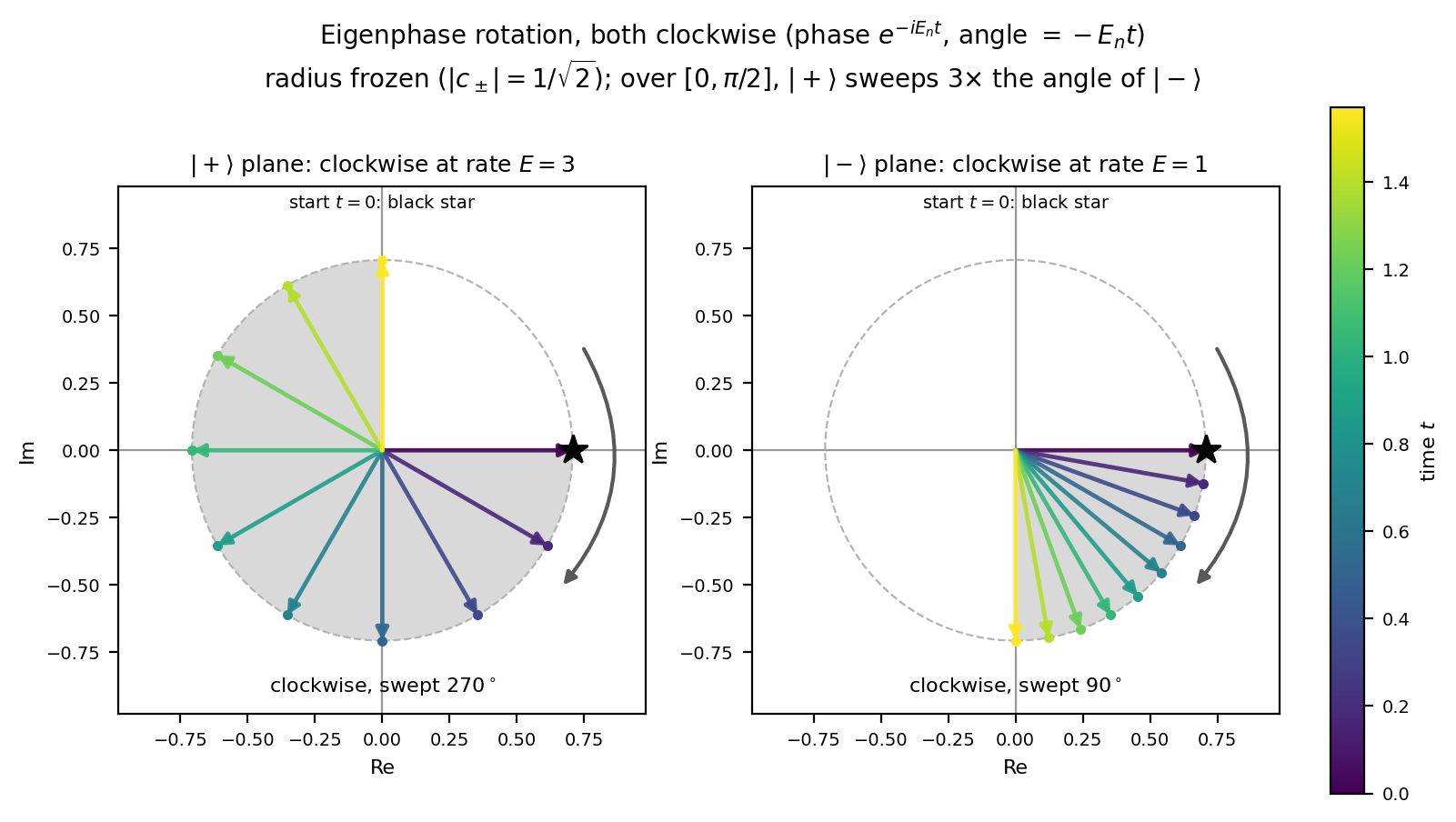
\(\mathbb{R}^4\) drawn as two \(\mathbb{R}^2\) Argand planes, one per eigendirection. Each eigen-component's arrow sweeps its circle of fixed radius \(1/\sqrt2\). Both rotate clockwise because the phase \(e^{-iE_n t}\) decreases the angle (\(-E_n t\)); over the interval shown, \(\lvert+\rangle\) sweeps three times the angle of \(\lvert-\rangle\) (the shaded sector, \(270^\circ\) versus \(90^\circ\)). Colour encodes time.

11.2 Reconstruction as interference

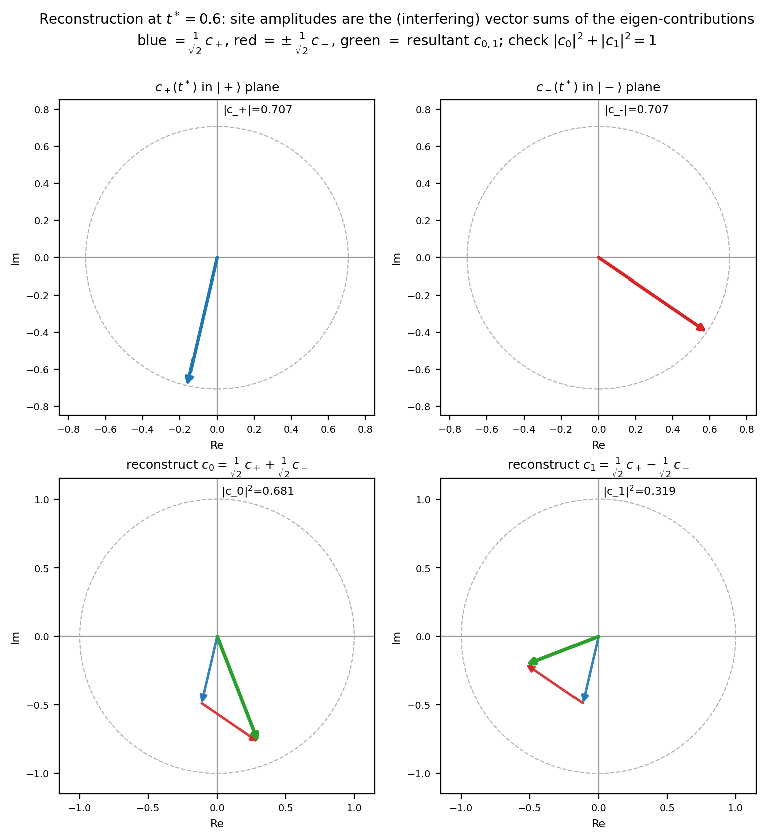
At \(t^*=0.6\), the site amplitudes are the vector sums of the eigen-contributions. \(c_0=\tfrac1{\sqrt2}c_++\tfrac1{\sqrt2}c_-\) adds nearly constructively (\(\lvert c_0\rvert^2=0.681\)); \(c_1=\tfrac1{\sqrt2}c_+-\tfrac1{\sqrt2}c_-\) adds nearly destructively (\(\lvert c_1\rvert^2=0.319\)); the two sum to 1. Interference as vector addition.

11.3 Two bases, two behaviors

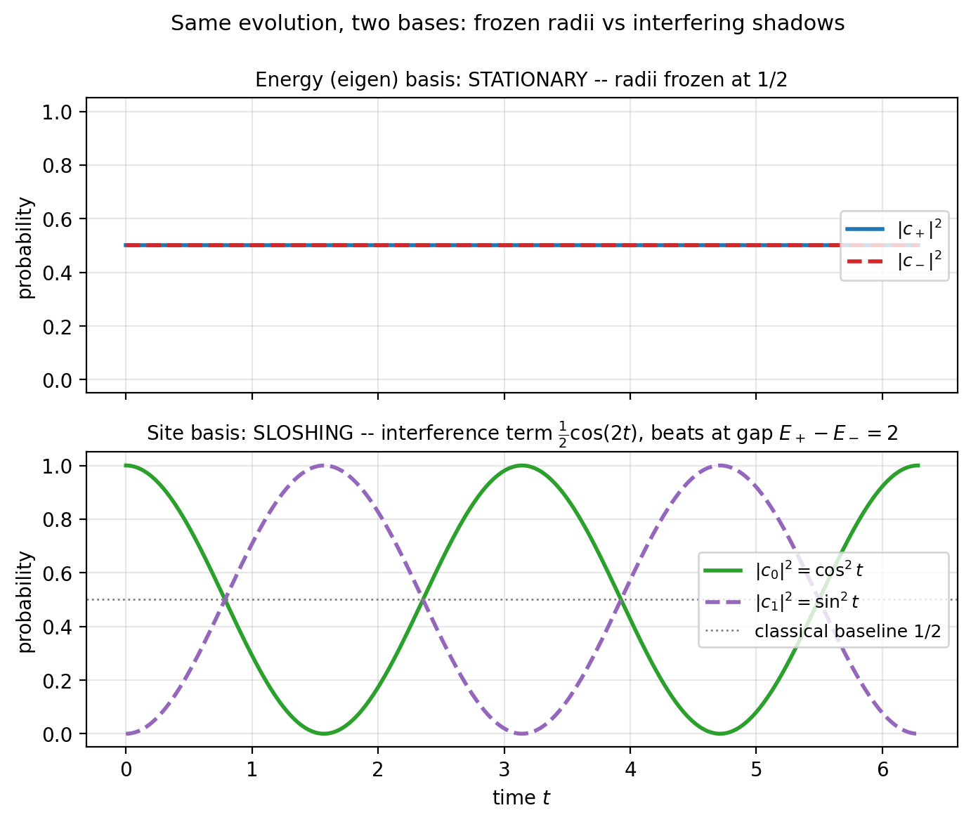
In the energy basis the probabilities are frozen at \(\tfrac12\) (stationary). In the site basis they slosh as \(\cos^2 t\) and \(\sin^2 t\); the interference term \(\tfrac12\cos(2t)\) beats at the gap \(E_+-E_-=2\).

11.4 Storyboard: rotation drives reconstruction

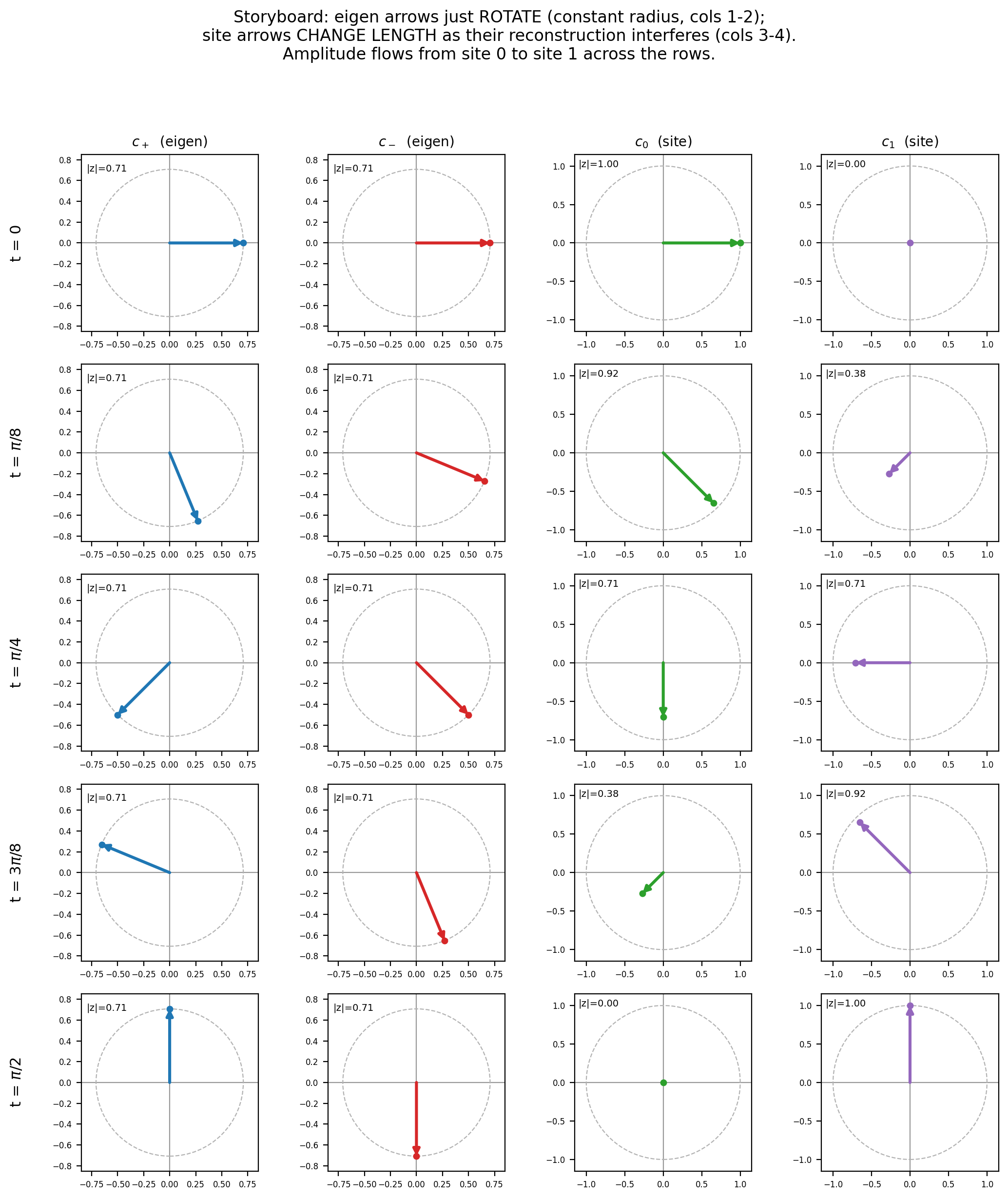
Five time-rows (\(t=0,\pi/8,\pi/4,3\pi/8,\pi/2\)) against four columns (\(c_+,c_-,c_0,c_1\)). The eigen arrows (columns 1 and 2) just rotate at constant radius \(0.71\); the site arrows (columns 3 and 4) change length as their reconstruction interferes, and amplitude flows from site 0 (\(c_0:1.00\to0.00\)) to site 1 (\(c_1:0.00\to1.00\)) down the rows. The same data, seen two ways.

---

12. The whole story in one paragraph

The matrix exponential is the scalar exponential's power series with a matrix substituted in, so \(e^{-iHt}\) solves \(\dot\psi=-iH\psi\) by term-by-term differentiation. The Hermitian hypothesis \(H=H^\dagger\) (equivalently \(\langle a\vert Hb\rangle=\langle Ha\vert b\rangle\)) guarantees a complete orthonormal eigenbasis with real eigenvalues, which lets \(H\) be written as a sum of shadow-casting projectors, \(H=\sum_n E_n\lvert n\rangle\langle n\rvert\), each eigendirection stretched by its real eigenvalue. Functions of \(H\) then act eigenvalue-by-eigenvalue, so the propagator is \(e^{-iHt}=\sum_n e^{-iE_n t}\lvert n\rangle\langle n\rvert\): the same eigendirections, now spun by pure phases (pure because the eigenvalues are real), which makes \(e^{-iHt}\) a unitary rotation of state space that conserves probability. The spin lives inside each coordinate's own Argand plane, one clock per eigendirection turning at rate \(E_n\), so on the energy basis the radii are frozen (stationary states) while on any other basis the phases interfere and probability sloshes at frequencies equal to energy gaps. And the entire difference between this quantum rotation and the familiar machine-learning picture of a symmetric matrix stretching a vector along its eigenaxes is a single factor of \(i\), which bends real stretch-eigenvalues \(e^{E_n t}\) onto the unit circle as phase-eigenvalues \(e^{-iE_n t}\).