Circuit Bench 03: Deutsch-Jozsa¶

What this circuit does¶

An algorithm that answers a yes-or-no question about a function in one query — a question that classically requires up to \(2^{n-1}+1\) queries in the worst case. This is the first Circuit Bench example of an exponential separation in deterministic query complexity.

Here's the setup: someone gives you a black box (an "oracle") that computes a function \(f:\{0,1\}^n \to \{0,1\}\). You're promised that \(f\) is either constant (same output for all inputs) or balanced (outputs 0 for exactly half the inputs, 1 for the other half). Which is it?

Classically, you might need to check just over half the inputs before you know. Quantumly: one shot.

Circuit components¶

3 qubits (2 input + 1 ancilla)
Hadamard gates (h)
CNOT gates (cx)
1 X gate (x)
A Quokka (puck or app)

Prerequisites: Circuit Bench 01 — Bell State. You should be comfortable with superposition and the Hadamard gate.

Files on the bench¶

Open the source directory on GitHub.

File	Purpose
`deutsch_jozsa_constant.qasm`	Run the algorithm with a constant-zero oracle
`deutsch_jozsa_balanced.qasm`	Run it with the balanced oracle \(f(x)=x_0\oplus x_1\)
`expected.txt`	Expected result and the constant/balanced decision rule
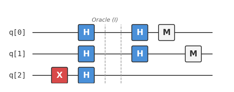
`circuit_constant.png`	Constant-oracle circuit diagram
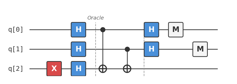
`circuit_balanced.png`	Balanced-oracle circuit diagram

Background: constant vs. balanced¶

Suppose \(f\) takes 2-bit inputs. There are \(2^2 = 4\) possible inputs: 00, 01, 10, 11.

Constant means \(f\) gives the same answer for all of them:

\(x\)	\(f(x) = 0\)
00	0
01	0
10	0
11	0

Balanced means exactly half give 0 and half give 1:

\(x\)	\(f(x) = x_0 \oplus x_1\)
00	0
01	1
10	1
11	0

With 2 bits, a classical algorithm needs at most 3 queries to be certain (if the first two outputs agree, you still don't know — a balanced function could match on those two). For \(n\) bits, the worst case is \(2^{n-1}+1\) queries.

The Deutsch-Jozsa algorithm: one query, any \(n\), 100% correct.

Circuit walkthrough¶

We'll run two versions: one with a constant oracle (\(f(x) = 0\), does nothing) and one with a balanced oracle (\(f(x) = x_0 \oplus x_1\), XOR of the input bits). The same algorithm, different oracles, different results.

Step 1: Prepare the ancilla in \(|{-}\rangle\)¶

x q[2];
h q[2];

This puts the ancilla qubit into \(|{-}\rangle = \frac{1}{\sqrt{2}}(|0\rangle - |1\rangle)\).

Why? Because of a trick called phase kickback. When the oracle flips the ancilla (computing \(|y \oplus f(x)\rangle\)), the \(|{-}\rangle\) state converts that bit flip into a phase on the input register:

\[|x\rangle|{-}\rangle \xrightarrow{U_f} (-1)^{f(x)}|x\rangle|{-}\rangle\]

The ancilla itself is unchanged. The oracle's effect has been "kicked back" as a phase \((-1)^{f(x)}\) on the input. This is the key insight — it turns a function evaluation into an interference pattern.

Step 2: Put the input register in superposition¶

h q[0];
h q[1];

The input register is now an equal superposition of all 4 basis states:

\[\frac{1}{2}(|00\rangle + |01\rangle + |10\rangle + |11\rangle)\]

Combined with the ancilla, the full state is:

\[\frac{1}{2}(|00\rangle + |01\rangle + |10\rangle + |11\rangle) \otimes |{-}\rangle\]

Step 3: Apply the oracle¶

Constant oracle (\(f(x) = 0\)):

// Do nothing — the constant-zero oracle is the identity

Since \(f(x) = 0\) for all \(x\), the phase is \((-1)^0 = 1\) for every term. Nothing changes.

Balanced oracle (\(f(x) = x_0 \oplus x_1\)):

cx q[0], q[2];
cx q[1], q[2];

Each CNOT flips the ancilla if the corresponding input bit is 1. The net effect: the ancilla is flipped if and only if \(x_0 \neq x_1\) — i.e., \(f(x) = x_0 \oplus x_1\). Thanks to phase kickback, this applies \((-1)^{x_0 \oplus x_1}\) to each input term:

\[\frac{1}{2}\Big[(-1)^0|00\rangle + (-1)^1|01\rangle + (-1)^1|10\rangle + (-1)^0|11\rangle\Big] \otimes |{-}\rangle\]

\[= \frac{1}{2}(|00\rangle - |01\rangle - |10\rangle + |11\rangle) \otimes |{-}\rangle\]

The signs encode \(f\).

Step 4: Hadamard the input register¶

h q[0];
h q[1];

The Hadamard transform "decodes" the sign pattern. This is where interference happens.

Constant oracle: The state before this step is \(\frac{1}{2}(|00\rangle + |01\rangle + |10\rangle + |11\rangle)\) — all phases positive. Applying \(H \otimes H\):

\[H^{\otimes 2} \cdot \frac{1}{2}(|00\rangle + |01\rangle + |10\rangle + |11\rangle) = |00\rangle\]

All terms interfere constructively into \(|00\rangle\).

Balanced oracle: The state is \(\frac{1}{2}(|00\rangle - |01\rangle - |10\rangle + |11\rangle)\). Applying \(H \otimes H\):

\[H^{\otimes 2} \cdot \frac{1}{2}(|00\rangle - |01\rangle - |10\rangle + |11\rangle) = |11\rangle\]

The negative phases cause destructive interference on \(|00\rangle\) and constructive interference on \(|11\rangle\).

Step 5: Measure the input register¶

measure q[0] -> c[0];
measure q[1] -> c[1];

Constant oracle → always 00: constructive interference piles all amplitude onto \(|00\rangle\).
Balanced oracle → never 00: destructive interference on \(|00\rangle\) means we always get something else. For our balanced function, we always get 11.

The rule: if the measurement is all zeros, the function is constant. If it's anything else, the function is balanced. One query. Done.

The complete circuits¶

Constant oracle (\(f(x) = 0\))¶

Available as deutsch_jozsa_constant.qasm:

OPENQASM 2.0;
include "qelib1.inc";

qreg q[3];   // q[0], q[1] = input; q[2] = ancilla
creg c[2];   // measure input register only

// Step 1: Ancilla in |−⟩
x q[2];
h q[2];

// Step 2: Input in superposition
h q[0];
h q[1];

// Step 3: Oracle f(x) = 0 — identity (do nothing)

// Step 4: Hadamard on input
h q[0];
h q[1];

// Step 5: Measure input
measure q[0] -> c[0];
measure q[1] -> c[1];

Balanced oracle (\(f(x) = x_0 \oplus x_1\))¶

Available as deutsch_jozsa_balanced.qasm:

OPENQASM 2.0;
include "qelib1.inc";

qreg q[3];   // q[0], q[1] = input; q[2] = ancilla
creg c[2];   // measure input register only

// Step 1: Ancilla in |−⟩
x q[2];
h q[2];

// Step 2: Input in superposition
h q[0];
h q[1];

// Step 3: Oracle f(x) = x0 XOR x1
cx q[0], q[2];
cx q[1], q[2];

// Step 4: Hadamard on input
h q[0];
h q[1];

// Step 5: Measure input
measure q[0] -> c[0];
measure q[1] -> c[1];

Circuit diagrams:

Constant:

q[0] : ─── H ─────────── H ─── M
q[1] : ─── H ─────────── H ─── M
q[2] : ─ X ─ H ──────────────────

Balanced:

q[0] : ─── H ──────●──── H ─── M
                    │
q[1] : ─── H ──────│──●─ H ─── M
                    │  │
q[2] : ─ X ─ H ────X──X──────────

Run it¶

Paste each circuit into your Quokka:

Constant oracle:

{'00': 1.0}

Always 00. The function is constant. ✓

Balanced oracle:

{'11': 1.0}

Always 11 — not 00, so the function is balanced. ✓

Try it: Modify the balanced oracle. Replace cx q[0], q[2]; cx q[1], q[2]; with just cx q[0], q[2]; (implementing \(f(x) = x_0\)). This is also balanced. What do you get? (Spoiler: 10 — still not 00, so the algorithm correctly identifies it.)

Extend and experiment¶

Build the other constant oracle. Add x q[2]; in the oracle section of deutsch_jozsa_constant.qasm. This implements \(f(x)=1\). The input register still measures 00 because constant zero and constant one differ only by a global phase in this algorithm.
Use a one-bit balanced oracle. In the balanced file, keep only one oracle CNOT. The exact non-zero output changes with the chosen input bit, but it is still never 00; the algorithm still classifies the function as balanced.
Remove the decoding Hadamards. Delete the two Hadamards after the oracle. All four input strings become approximately equally likely because the function is still encoded in phase and has not been converted into a measurement pattern.

Analysis¶

Phase kickback — the mechanism behind the magic

Phase kickback is the single most important trick in quantum computing. Let's unpack it.

An oracle \(U_f\) acts as: \(U_f|x\rangle|y\rangle = |x\rangle|y \oplus f(x)\rangle\). If the ancilla is \(|{-}\rangle = \frac{1}{\sqrt{2}}(|0\rangle - |1\rangle)\):

\[U_f|x\rangle|{-}\rangle = |x\rangle \cdot \frac{1}{\sqrt{2}}(|0 \oplus f(x)\rangle - |1 \oplus f(x)\rangle)\]

Case \(f(x) = 0\):

\[|x\rangle \cdot \frac{1}{\sqrt{2}}(|0\rangle - |1\rangle) = |x\rangle|{-}\rangle\]

No change. Phase \(= +1\).

Case \(f(x) = 1\):

\[|x\rangle \cdot \frac{1}{\sqrt{2}}(|1\rangle - |0\rangle) = -|x\rangle|{-}\rangle\]

The ancilla returns to \(|{-}\rangle\), but a global minus sign appears. This is the kickback: the oracle's effect on the ancilla has been transferred to a phase on the input register.

In general: \(U_f|x\rangle|{-}\rangle = (-1)^{f(x)}|x\rangle|{-}\rangle\).

The ancilla is unchanged (it's still \(|{-}\rangle\)). The information about \(f(x)\) lives entirely in the phase of \(|x\rangle\). This is why we don't measure the ancilla — it's done its job.

Phase kickback appears again in Bernstein-Vazirani (Circuit Bench 04), Simon's algorithm (Circuit Bench 05), Grover's search (Circuit Bench 06), and in a more sophisticated form in quantum phase estimation (Circuit Bench 10). Master it here.

The Hadamard transform as Fourier analysis

Why does applying Hadamards after the oracle reveal whether \(f\) is constant or balanced?

The \(n\)-qubit Hadamard transform is:

\[H^{\otimes n}|x\rangle = \frac{1}{\sqrt{2^n}} \sum_{z \in \{0,1\}^n} (-1)^{x \cdot z} |z\rangle\]

where \(x \cdot z = x_0 z_0 \oplus x_1 z_1 \oplus \cdots\) is the bitwise inner product.

After the oracle (with phase kickback), the input register is:

\[\frac{1}{\sqrt{2^n}} \sum_x (-1)^{f(x)} |x\rangle\]

Applying \(H^{\otimes n}\) again:

\[H^{\otimes n} \cdot \frac{1}{\sqrt{2^n}} \sum_x (-1)^{f(x)} |x\rangle = \frac{1}{2^n} \sum_z \left(\sum_x (-1)^{f(x) + x \cdot z}\right) |z\rangle\]

The amplitude of \(|00\ldots0\rangle\) (i.e., \(z = 0\)) is:

\[\alpha_0 = \frac{1}{2^n} \sum_x (-1)^{f(x)}\]

Constant \(f\): All \((-1)^{f(x)}\) terms have the same sign. The sum is \(\pm 2^n\). So \(|\alpha_0|^2 = 1\).
Balanced \(f\): Half the terms are \(+1\), half are \(-1\). The sum is \(0\). So \(|\alpha_0|^2 = 0\).

This is why measuring all zeros means constant, and any non-zero result means balanced. It's Fourier analysis: the Hadamard transform computes the "DC component" of \((-1)^{f(x)}\), which is nonzero only for constant functions.

Classical lower bound: why this speedup is real

Deterministic: A classical algorithm that queries \(f\) one input at a time needs \(2^{n-1} + 1\) queries in the worst case to distinguish constant from balanced. After seeing \(2^{n-1}\) identical outputs, you still can't rule out a balanced function (the other half could all be different). One more query settles it.

Randomised: A randomised classical algorithm can do better — after \(k\) queries that all return the same value, the probability that \(f\) is balanced (assuming a uniform prior) is at most \(1/2^{k-1}\). So \(O(\log(1/\epsilon))\) queries suffice for confidence \(1 - \epsilon\). But this is probabilistic; Deutsch-Jozsa is exact.

Quantum: One query. No probability of error. This is a provable (not heuristic) exponential separation between deterministic classical and quantum query complexity.

The caveat: this is a separation in the query model, not in total computation time. The function is given as a black box. In practice, if you know the structure of \(f\), classical algorithms might exploit that structure. The Deutsch-Jozsa problem is artificial — but the techniques it introduces (phase kickback, Hadamard Fourier transform) are the machinery behind algorithms that solve real problems.

From Deutsch to Deutsch-Jozsa

David Deutsch's original 1985 algorithm was the \(n = 1\) case: one input bit, one oracle query. The function \(f:\{0,1\} \to \{0,1\}\) is either constant (\(f(0) = f(1)\)) or balanced (\(f(0) \neq f(1)\)). Deutsch showed a quantum computer can distinguish them in one query.

Deutsch and Jozsa generalised this to \(n\) bits in 1992. The algorithm is essentially the same — the Hadamard transform scales naturally. But the speedup grows from a factor of 2 (for \(n = 1\)) to an exponential separation (for general \(n\)).

The Deutsch-Jozsa algorithm is historically important: it was the first problem shown to have an exponential quantum speedup (in the query model). It directly inspired Simon's algorithm (Circuit Bench 05), which in turn inspired Shor's algorithm for factoring.

Practical notes¶

Phase kickback is the technique to internalise. It appears in nearly every quantum algorithm: Bernstein-Vazirani, Simon, Grover, QPE. If you understand why the \(|{-}\rangle\) ancilla converts bit flips to phases, you understand a core piece of quantum computing.
We don't measure the ancilla. The ancilla stays in \(|{-}\rangle\) throughout — it's a catalyst. Only the input register carries information about \(f\), encoded in phases. This is a recurring pattern.
Try building your own oracle. Any balanced function works. For 2 bits, some options: \(f(x) = x_0\) (CNOT from q[0] to q[2]), \(f(x) = x_1\) (CNOT from q[1] to q[2]), \(f(x) = x_0 \oplus x_1 \oplus 1\) (add an X gate on q[2] after the CNOTs). Run each one and verify you never get 00.
If you liked this, try: Circuit Bench 04 (Bernstein-Vazirani) uses the exact same circuit structure but extracts more information — not just "constant or balanced?" but the actual hidden string. It's a direct upgrade.