Circuit Bench 09: Quantum Fourier Transform
The Quantum Fourier Transform, or QFT, is the circuit that lets a quantum register listen for periodic structure.
That sentence is more useful than the usual one.
The usual description says that the QFT is the quantum version of the discrete Fourier transform. That is true, but it can also mislead. A classical Fourier transform gives you a list of coefficients you can read. A QFT changes the amplitudes and phases of a quantum state. When you measure immediately afterwards, you only get one bit string.
So the QFT is not powerful because it prints a Fourier spectrum.
It is powerful because, inside a larger circuit, it can turn a phase pattern into a measurement pattern.
What this circuit does
This note builds a three-qubit QFT on the computational-basis input \(|5\rangle\), which is binary 101.
The mathematical action is:
where \(N = 2^n\) for an \(n\)-qubit register.
For this circuit, \(n = 3\) and \(N = 8\). Every output basis state has probability \(1/8\). The information about the input is in the relative phases, not in the raw Z-basis probabilities.
That is the first important lesson: a standalone QFT on a basis state looks uniform when measured.
Prerequisites
If gates, measurement, and basis changes are new, start with Circuit Bench 00: Reading a Quantum Circuit.
For this note, you only need three circuit ideas:
- A Hadamard gate creates a one-qubit superposition.
- A controlled phase gate changes phase only when both its control and target are
1. - A final measurement in the computational basis can see probability, but not phase directly.
OpenQASM 2.0 names the controlled phase gate cu1(theta) control, target;. In newer SDKs you may also see the same idea written as cp(theta).
Files on the bench
Open the source directory on GitHub.
| File | Purpose |
|---|---|
qft.qasm |
Apply a three-qubit QFT to the basis state \(\lvert101\rangle\) |
expected.txt |
Expected uniform Z-basis counts and their interpretation |
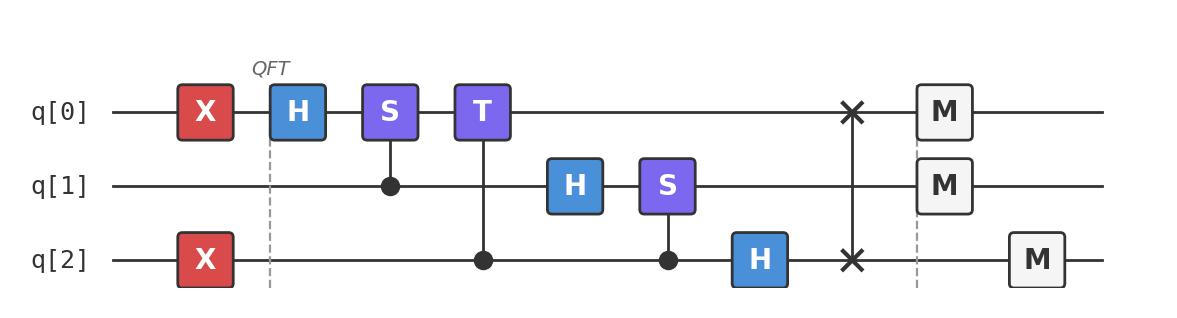
circuit.png |
QFT circuit diagram |
Circuit walkthrough
1. Prepare the input
The circuit prepares the three-qubit basis state 101:
This is the state \(|5\rangle\) under the bit-ordering used by the note.
2. Apply the QFT rotations
The QFT is built from Hadamards and controlled phase rotations:
The Hadamards create equal-magnitude branches. The controlled phase gates add the fine-grained roots of unity that distinguish a Fourier transform from a plain Hadamard transform.
The angles are:
| Angle | Meaning |
|---|---|
| \(\pi/2\) | controlled \(R_2\) phase |
| \(\pi/4\) | controlled \(R_3\) phase |
Each later qubit controls a smaller phase rotation on the earlier qubits. That pattern is what lets the QFT encode binary phase information efficiently.
3. Fix the output order
The textbook QFT circuit naturally reverses the output order. The final swap puts the register back into the displayed order:
4. Measure
For a computational-basis input, measurement should be close to uniform across the eight possible bit strings.
The complete circuit
Available as qft.qasm:
OPENQASM 2.0;
include "qelib1.inc";
qreg q[3];
creg c[3];
// Input: |5> = |101> in displayed order q[0] q[1] q[2]
x q[0];
x q[2];
// QFT on 3 qubits
h q[0];
cu1(1.5708) q[1], q[0];
cu1(0.7854) q[2], q[0];

h q[1];
cu1(1.5708) q[2], q[1];

h q[2];
// Restore displayed bit order
swap q[0], q[2];
measure q[0] -> c[0];
measure q[1] -> c[1];
measure q[2] -> c[2];
Run it
Paste qft.qasm into Quokka. With 1024 shots, you should see all eight bit strings with roughly equal counts:
000: about 128
001: about 128
010: about 128
011: about 128
100: about 128
101: about 128
110: about 128
111: about 128
Do not read that as "the QFT lost the information." The information is in phase. A computational-basis measurement is simply the wrong instrument for seeing it directly.
Extend and experiment
- Change the basis-state input. Move or remove the two preparation X gates to try
000or001; to prepare111, keep both existing X gates and addx q[1];. Every computational-basis input still produces a uniform Z-basis distribution after the QFT. The inputs differ in phase, which these counts do not reveal. - Remove the final swap. The measured distribution remains uniform. This shows that Z-basis counts cannot validate the output ordering of a standalone QFT on a basis state, even though that ordering matters when the QFT is used inside another algorithm.
- Append the inverse QFT. Before measurement, add the inverse sequence:
swap q[0], q[2], thenh q[2], controlled phases-pi/2fromq[2]toq[1],h q[1], controlled phases-pi/4fromq[2]toq[0]and-pi/2fromq[1]toq[0], thenh q[0]. The QFT followed by its inverse should recover101deterministically in an ideal run.
What this shows
This circuit shows the shape of the QFT:
- Hadamards spread amplitude across the whole register.
- Controlled phase rotations encode a Fourier phase pattern.
- A basis-state input produces equal output probabilities.
- The useful information is invisible to direct Z-basis measurement.
That last point is why the QFT usually appears as a subroutine. In quantum phase estimation, the inverse QFT turns a phase pattern into a bit string. In Shor's algorithm, that bit string is then processed classically to recover a period.
What this does not show
This circuit does not produce a readable Fourier spectrum. If you measure once, you get one bit string. If you measure many times, you see a distribution.
The QFT is exponentially smaller than applying a classical FFT to an explicitly stored \(2^n\)-component vector: it uses \(O(n^2)\) gates rather than \(O(n2^n)\) arithmetic operations. But that comparison has a catch. The quantum state is not a classical array you can print. The QFT is useful when an algorithm only needs a small amount of global Fourier information, such as a phase or a period.
For the circuit that turns that hidden phase into a measured value, continue to Circuit Bench 10: Quantum Phase Estimation.