Circuit Bench 12: Quantum Counting
What this circuit does
An algorithm that counts the number of solutions to a search problem — without finding them. Given the same oracle from Grover's search (Circuit Bench 06), quantum counting tells you how many items match, using QPE (Circuit Bench 10) on the Grover operator.
This is the capstone of the Circuit Bench sequence: it combines everything we've built. Grover's oracle defines the problem. The Grover operator encodes the answer in its eigenvalues. QPE extracts the eigenvalue. And the QFT (inside QPE) provides the precision.
Circuit components
- 4 qubits (2 counting + 2 search)
- Hadamard gates (
h) - Toffoli gates (
ccx) - Controlled-Z gates (
cz) - X gates (
x) - Controlled phase gate (
cp) - SWAP gate (
swap) - A Quokka (puck or app)
Prerequisites: Circuit Bench 06 — Grover's Search and Circuit Bench 10 — QPE.
Files on the bench
Open the source directory on GitHub.
| File | Purpose |
|---|---|
quantum_counting.qasm |
Estimate the number of marked states with two counting qubits |
expected.txt |
Expected coarse phase distribution and inferred count |
circuit.png |
Controlled-Grover and inverse-QFT circuit diagram |
Background: why count instead of search?
Grover's search finds a solution in \(O(\sqrt{N/M})\) queries — but you need to know \(M\) (the number of solutions) to choose the right number of iterations. Too few and you haven't amplified enough; too many and you overshoot.
Quantum counting solves this chicken-and-egg problem. It estimates \(M\) directly, which then tells you the optimal number of Grover iterations:
More broadly, counting is interesting in its own right. Many practical questions are counting problems:
- How many valid configurations satisfy these constraints?
- How many database entries match this query?
- What fraction of the search space contains solutions?
How it works
The Grover operator's eigenvalues
The Grover operator \(G = D \cdot O\) (diffusion × oracle) has eigenvalues \(e^{\pm 2i\theta}\) where:
If we can estimate \(\theta\), we can recover \(M = N\sin^2(\theta)\).
QPE on \(G\)
Apply quantum phase estimation with: - Unitary: \(G\) (the Grover operator) - Eigenstate: \(|s\rangle = H^{\otimes n}|0\rangle^{\otimes n}\) (the uniform superposition, which is close to the Grover eigenspace) - Counting qubits: \(t\) qubits for \(t\)-bit precision on \(\theta\)
The counting register will encode \(\theta/\pi\), from which we extract \(M\).
Circuit walkthrough
We'll count the number of solutions to a 2-qubit search with oracle marking \(|11\rangle\). So \(N = 4\) and \(M = 1\).
Step 1: Initialize
h q[0]; h q[1];    // counting register in superposition
h q[2]; h q[3];    // search register in uniform superposition
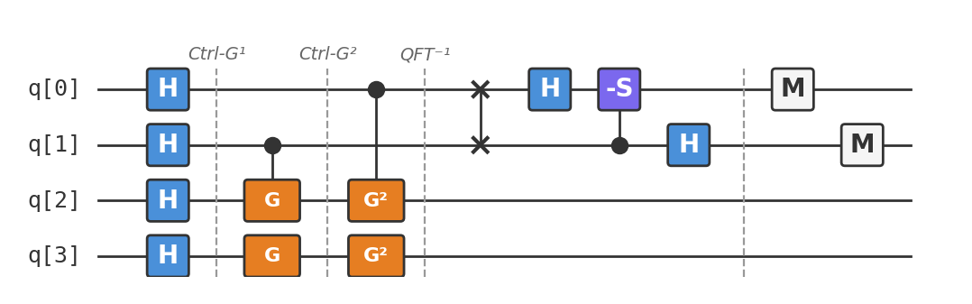
Step 2: Controlled Grover iterations
Each counting qubit controls \(G^{2^k}\) on the search register:
- \(q[1]\) (LSB) controls \(G^1\)
- \(q[0]\) (MSB) controls \(G^2\)
Each Grover iteration consists of: 1. Oracle: Phase-flip the marked state \(|11\rangle\) 2. Diffusion: Reflect about the uniform superposition
The controlled versions are implemented using Toffoli gates and controlled-Z gates.
Step 3: Inverse QFT
This converts the phase-encoded \(\theta\) to a bit string in the counting register.
Step 4: Measure
Read the counting register and compute \(\hat{\theta} = \pi \cdot (\text{result}) / 2^t\), then \(\hat{M} = N \sin^2(\hat{\theta})\).
The complete circuit
Available as quantum_counting.qasm. The circuit is the longest on the Circuit Bench — it combines QPE's structure with Grover's oracle and diffusion as the controlled unitary.
Run it
Paste quantum_counting.qasm into your Quokka. With 2 counting qubits, the resolution is coarse:
The dominant outcome is \(01\) (decimal 1), giving: - \(\hat{\theta} = \pi \times 1/4 = \pi/4\) - \(\hat{M} = 4 \times \sin^2(\pi/4) = 4 \times 0.5 = 2\)
This isn't exact (\(M = 1\), not 2) — we only have 2 counting qubits! With 3 counting qubits, the estimate improves significantly. With \(t\) counting qubits, the error in \(M\) is \(O(\sqrt{M}/2^t)\).
More counting qubits = better precision
The precision scales as \(1/2^t\). For practical problems:
- \(t = 4\) qubits: resolve \(M\) to about \(N/16\)
- \(t = 8\) qubits: resolve \(M\) to about \(N/256\)
- \(t = \lceil\log_2 N\rceil + 4\): typically sufficient for good estimates
Extend and experiment
- Change the shot count. Run 128, 1024, and 8192 shots. The sampled frequencies become more stable, but the two-qubit phase grid remains spaced by \(1/4\). Shots reduce sampling error; they do not improve phase resolution.
- Remove the inverse-QFT phase gate. Delete
cp(-1.5708) q[1], q[0];and compare the counting-register distribution. The remaining Hadamards no longer decode the phase with the same two-bit QFT, so the usual mapping from bit string to \(\hat M\) is no longer valid. - Design a three-bit counter. Add a third counting qubit, a controlled-\(G^4\) block, and a three-qubit inverse QFT. The phase grid becomes twice as fine, but the largest controlled power doubles the Grover work and makes the circuit deeper. Record both the improved ideal estimate and the extra noise on hardware; this is the precision-cost tradeoff that the four-qubit demonstration omits.
Analysis
Eigenvalues of the Grover operator
The Grover operator \(G = (2|\psi\rangle\langle\psi| - I)(I - 2|w\rangle\langle w|)\) acts on the 2D subspace spanned by \(|w\rangle\) (marked states) and \(|w^\perp\rangle\) (unmarked states).
In the \(\{|w\rangle, |w^\perp\rangle\}\) basis, \(G\) is a rotation by angle \(2\theta\):
where \(\sin\theta = \sqrt{M/N}\).
The eigenvalues are \(e^{\pm 2i\theta}\) with eigenvectors:
The initial state \(|\psi\rangle = \sin\theta|w\rangle + \cos\theta|w^\perp\rangle\) is:
QPE on \(|\psi\rangle\) returns \(+2\theta\) or \(-2\theta\) with equal probability. Both give the same \(|\sin^2\theta| = M/N\).
Error analysis: precision vs counting qubits
With \(t\) counting qubits, the phase resolution is \(\delta\theta = \pi/2^t\). The error in \(M\) is:
For \(M\) to be estimated to \(\pm 1\):
For \(N = 4\): \(t \geq 5\) for exact counting. Our 2-qubit demo is deliberately coarse to keep the circuit small enough to inspect.
In practice, you often don't need exact \(M\) — an estimate within a constant factor suffices to choose the right number of Grover iterations. Even \(t = \lceil\log_2\sqrt{N}\rceil\) extra qubits gives useful information.
Application: optimal Grover search without knowing \(M\)
The Boyer-Brassard-Høyer-Tapp (BBHT) algorithm uses quantum counting to make Grover's search optimal:
- Run quantum counting with \(t\) counting qubits to estimate \(\hat{M}\)
- Set \(k = \lfloor\frac{\pi}{4}\sqrt{N/\hat{M}}\rfloor\)
- Run Grover's search with \(k\) iterations
Total query complexity: \(O(\sqrt{N/M})\) — optimal, even without knowing \(M\) in advance.
The counting step costs \(O(\sqrt{N})\) queries (dominated by the controlled-\(G^{2^{t-1}}\) operation), which is no worse than the search itself.
For comparison, the naive approach (guess \(M\), run Grover's, check, repeat with doubled guess) also achieves \(O(\sqrt{N/M})\) but with worse constants.
Quantum counting for #SAT and counting problems
Quantum counting can estimate the number of satisfying assignments to a Boolean formula:
- Encode the formula as a Grover oracle (marks satisfying assignments)
- Run quantum counting on the oracle
- Get \(\hat{M}\) ≈ number of satisfying assignments
This gives a quadratic speedup for counting: classical counting for #SAT takes \(O(2^n)\) time in the worst case; quantum counting takes \(O(2^{n/2})\).
While this doesn't make #SAT easy (it's #P-hard classically, and the quantum speedup is "only" quadratic), it's significant for approximate counting. Many practical problems — estimating partition functions, counting independent sets, computing volumes — benefit from even a quadratic improvement.
The full picture: Circuit Bench 06 + 09 + 10 + 12
Quantum counting is the capstone that ties together three earlier Circuit Bench notes:
| Component | Circuit Bench | Role in Quantum Counting |
|---|---|---|
| Grover operator | Circuit Bench 06 | The unitary whose eigenvalue encodes \(M\) |
| QFT | Circuit Bench 09 | The final step of QPE (inverse QFT) |
| QPE | Circuit Bench 10 | The framework that extracts the eigenvalue |
| Quantum Counting | Circuit Bench 12 | The full algorithm |
The composition: QPE wraps the Grover operator, using the inverse QFT to read out \(\theta\). The angular resolution is set by the number of counting qubits. The answer gives \(M = N\sin^2(\theta)\).
This is the hidden subgroup / phase estimation paradigm at its most general. The same architecture — controlled unitary + inverse QFT — appears in Shor's algorithm (with modular exponentiation instead of Grover), quantum chemistry (with Hamiltonian simulation instead of Grover), and quantum simulation (with time-evolution operators).
Practical notes
-
This is the most complex circuit on the Circuit Bench. It combines controlled Grover iterations (oracle + diffusion) with QPE infrastructure (Hadamards, controlled powers, inverse QFT). The qubit count is small but the gate depth is significant.
-
2 counting qubits is coarse. Our demo uses \(t = 2\) to keep the circuit manageable. The estimate of \(M\) is approximate. In practice, you'd use more counting qubits (and more search qubits for a bigger search space).
-
The connection to Shor. Replace the Grover operator with modular exponentiation, and quantum counting becomes order-finding — the core of Shor's factoring algorithm. Same QPE wrapper, different unitary.
-
Congratulations — you've completed the Circuit Bench sequence! You now understand entanglement (Bell state), quantum communication (teleportation), quantum speedups (Deutsch-Jozsa through Simon), search (Grover), optimization (QAOA, VQE), the Fourier transform (QFT), eigenvalue estimation (QPE), noise mitigation (ZNE), and counting. These are the building blocks of all quantum algorithms.