Circuit Bench 07: QAOA for MaxCut
What this circuit does
A three-qubit QAOA circuit for MaxCut on a triangle.
If you came here from The $50M Delivery Route, this is the same teaching example viewed from the Circuit Bench. The blog post explains why a tiny graph belongs in a logistics story. This note does the narrower job: show the actual OpenQASM circuit, explain the gates, and tell you what to expect when you run it.
QAOA is a variational quantum algorithm. A quantum circuit prepares a probability distribution over candidate solutions; a classical optimiser chooses the circuit angles that make better solutions more likely. In this circuit note we use fixed angles that are already tuned for the triangle, so you can inspect the circuit without also building the optimiser.
Circuit components
- 3 qubits, one per graph node
- Hadamard gates (
h) - CNOT gates (
cx) - Z-rotations (
rz) - X-rotations (
rx) - Measurement
- A Quokka puck or app
Useful side paths: Circuit Bench 00 — Reading a Quantum Circuit covers gates, unitary rotations, and measurement bases; Circuit Bench 01 — Bell State covers Hadamard, CNOT, and measurement correlation in the first two-qubit example.
Files on the bench
Open the source directory on GitHub.
| File | Purpose |
|---|---|
qaoa_maxcut.qasm |
Run the tuned depth-1 triangle MaxCut circuit |
expected.txt |
Expected concentration on the six optimal cuts |
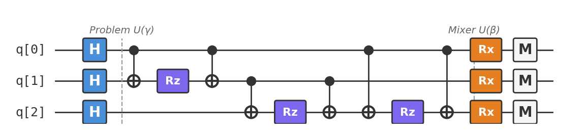
circuit.png |
Circuit diagram with problem and mixer layers |
The graph
We use the smallest graph that still shows the QAOA mechanism:
The edges are:
A bit string assigns each node to one side of the cut:
An edge is cut if its endpoints have different bits.
| Bit string | Cut value |
|---|---|
000 |
0 |
001 |
2 |
010 |
2 |
011 |
2 |
100 |
2 |
101 |
2 |
110 |
2 |
111 |
0 |
The best possible cut value is 2. Six bit strings achieve it; 000 and 111 cut no edges.
The circuit rhythm
Depth-1 QAOA has four stages:
- Prepare all colourings. Apply Hadamards to create an equal superposition over the eight bit strings.
- Apply one phase block per edge. Use a CNOT-
rz-CNOT sandwich to add a phase that depends on whether two endpoint bits agree or differ. - Mix neighbouring colourings. Apply
rxrotations so amplitude can move between bit strings that differ by one bit. - Measure. Sample a bit string and score its cut value.
The cost phase alone does not change measurement probabilities. It writes information into phase. The mixer is what lets those phases interfere and change the final probability distribution.
Parameter convention
OpenQASM 2.0 defines:
This note uses the same convention as the companion notebook:
For this triangle instance, the fixed angles are:
So the QASM uses:
Do not treat those numbers as universal QAOA constants. They are good angles for this particular graph and this particular gate convention.
Step 1: Prepare the search space
This creates an equal superposition over all eight possible cuts.
Step 2: Add one edge phase block per edge
For edge (0, 1):
The first CNOT computes the parity of the two endpoint bits into the target qubit. The rz gate applies a phase based on that parity. The second CNOT uncomputes the parity so the bit string is restored.
Repeat the same pattern for (0, 2) and (1, 2).
Step 3: Mix
The mixer lets amplitude flow between neighbouring bit strings. Because the edge blocks have already given different phases to different cut values, this mixing turns hidden phase information into visible probability bias.
Step 4: Measure
Each shot returns one candidate cut.
The complete circuit
The full QASM file is qaoa_maxcut.qasm:
OPENQASM 2.0;
include "qelib1.inc";
qreg q[3];
creg c[3];
h q[0];
h q[1];
h q[2];
cx q[0], q[1];
rz(2.528982) q[1];
cx q[0], q[1];
cx q[0], q[2];
rz(2.528982) q[2];
cx q[0], q[2];
cx q[1], q[2];
rz(2.528982) q[2];
cx q[1], q[2];
rx(0.612611) q[0];
rx(0.612611) q[1];
rx(0.612611) q[2];
measure q[0] -> c[0];
measure q[1] -> c[1];
measure q[2] -> c[2];
Run it
Paste qaoa_maxcut.qasm into Quokka and sample it.
In an ideal simulation with the fixed angles above, the six optimal bit strings are strongly favoured and 000 and 111 are heavily suppressed:
Shot noise means your exact counts will vary. The important thing to check is not the order of the bit strings; it is whether the samples are concentrated on cuts with value 2.
Extend and experiment
- Set every rotation angle to zero. Replace all
rzandrxangles with 0. The CNOT pairs cancel, the mixer is the identity, and the output returns to the uniform distribution: each string has probability \(1/8\), so the six optimal cuts receive 75% in total. - Remove only the mixer. Keep the three cost-phase blocks but set the
rxangles to 0. The Z-basis distribution is still uniform because diagonal phase gates alone cannot change computational-basis probabilities. This is the clean control for the mixer's role. - Sweep the QASM angles. Vary the three
rzvalues together around2.528982and the threerxvalues together around0.612611. For each pair, record the fraction of shots with cut value 2. Remember that the file stores \(2\gamma\) and \(2\beta\), not \(\gamma\) and \(\beta\) themselves.
Analysis
Why the CNOT-RZ-CNOT block is a ZZ phase
CNOT computes parity. For two bits \(a\) and \(b\), the target becomes \(a \oplus b\) after the first CNOT.
The rz rotation applies one phase when that parity is 0 and another phase when it is 1.
The second CNOT restores the target bit. The computational basis state is unchanged, but it has picked up a phase depending on whether the two endpoint bits agreed or differed.
Algebraically:
Setting \(\theta = 2\gamma\) gives the edge phase used in this note.
Where the optimiser went
Full QAOA does not normally start with fixed angles. It runs a loop:
choose gamma, beta
run the circuit many times
estimate the average cut value
update gamma, beta classically
repeat
This note freezes the loop at one good pair of angles so the circuit is readable as a standalone QASM program.
The companion notebook runs the same idea in a more workbook-like form: it builds the graph, brute-forces the answer, constructs QASM, samples the circuit, and sweeps the parameter landscape.
Practical notes
- This is a circuit note, not an advantage claim. The triangle does not need a quantum computer. It is small enough to expose the mechanism.
- The angles are convention-dependent. If you change signs, factors of two, or edge-order conventions, the best numerical angles can change.
- The optimiser is part of QAOA. This QASM file shows one tuned circuit. The full algorithm is the quantum-classical loop around it.
- MaxCut is the clean specimen. Scheduling, routing, and other optimisation problems need more elaborate encodings, but the pattern is the same: turn the objective into phases, mix, measure, and tune.