Circuit Bench 10: Quantum Phase Estimation
Quantum Phase Estimation, or QPE, is the circuit pattern that turns an eigenphase into bits.
That sounds abstract, so here is the concrete promise. Suppose a unitary operation \(U\) has an eigenstate \(|u\rangle\):
The number \(\varphi\) is a phase fraction between 0 and 1. QPE estimates that fraction. With three counting qubits, the circuit can report one of eight fractions:
This note estimates the phase of the \(T\) gate on the eigenstate \(|1\rangle\).
What this circuit does
The \(T\) gate is:
Since
the phase fraction is:
With three counting qubits, \(1/8\) is exactly representable. This note reads the counting register in displayed order q[0] q[1] q[2], so the ideal circuit returns the bit string 001, which is the integer 1, meaning:
Prerequisites
If the circuit vocabulary is new, start with Circuit Bench 00: Reading a Quantum Circuit.
If the inverse QFT step feels mysterious, read Circuit Bench 09: Quantum Fourier Transform. QPE works by creating a Fourier-like phase pattern and then using the inverse QFT to turn that pattern into a computational-basis state.
OpenQASM 2.0 writes the controlled phase operation as cu1(theta) control, target;.
Files on the bench
Open the source directory on GitHub.
| File | Purpose |
|---|---|
qpe.qasm |
Estimate the \(T\)-gate eigenphase \(\varphi=1/8\) |
expected.txt |
Expected three-bit phase estimate |
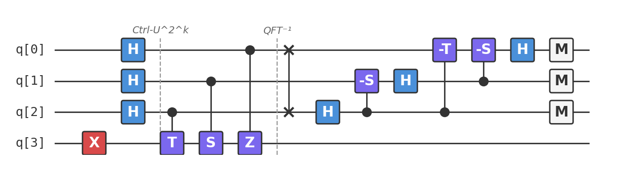
circuit.png |
QPE circuit diagram |
Circuit walkthrough
1. Prepare the eigenstate
The target qubit is q[3]. We prepare it in \(|1\rangle\), an eigenstate of \(T\):
2. Put the counting register into superposition
The counting register is q[0], q[1], and q[2], read in that displayed order:
This creates a superposition over the eight possible three-bit inputs.
3. Apply controlled powers of the unitary
QPE applies controlled versions of \(U^{2^k}\). Here \(U = T\), so the powers are simple phase gates. In the displayed register order, q[2] is the least significant counting qubit:
cu1(0.7854) q[2], q[3]; // controlled T
cu1(1.5708) q[1], q[3]; // controlled T^2 = controlled S
cu1(3.1416) q[0], q[3]; // controlled T^4 = controlled Z
Because the target is the eigenstate \(|1\rangle\), these gates kick phase back onto the counting register. After this step, the counting register contains the phase pattern for \(\varphi = 1/8\).
This is the part of QPE that matters most: the circuit has not measured the phase yet. It has written the phase into interference.
4. Apply the inverse QFT
The inverse QFT converts the phase pattern into a basis state:
swap q[0], q[2];
h q[2];
cu1(-1.5708) q[2], q[1];
h q[1];
cu1(-0.7854) q[2], q[0];
cu1(-1.5708) q[1], q[0];
h q[0];
For this exact phase, the counting register becomes 001.
5. Measure
The measured integer is 1, so the estimated phase is \(1/8\).
The complete circuit
Available as qpe.qasm:
OPENQASM 2.0;
include "qelib1.inc";
qreg q[4];
creg c[3];
// q[0..2] = counting register, displayed as q[0] q[1] q[2]
// q[3] = eigenstate register
// Prepare eigenstate |1> of the T gate
x q[3];
// Counting register superposition
h q[0];
h q[1];
h q[2];
// Controlled powers of T. The phase is phi = 1/8.
cu1(0.7854) q[2], q[3];
cu1(1.5708) q[1], q[3];
cu1(3.1416) q[0], q[3];
// Inverse QFT on the counting register
swap q[0], q[2];
h q[2];
cu1(-1.5708) q[2], q[1];
h q[1];
cu1(-0.7854) q[2], q[0];
cu1(-1.5708) q[1], q[0];
h q[0];
measure q[0] -> c[0];
measure q[1] -> c[1];
measure q[2] -> c[2];
Run it
Paste qpe.qasm into Quokka. With an ideal simulator, all shots should land on:
With 1024 shots, the expected result is approximately:
That bit string means integer 1 out of 8 possible three-bit values, so the recovered phase is \(1/8\).
Extend and experiment
- Use the zero-phase eigenstate. Remove
x q[3];, leaving the target in \(|0\rangle\). Since \(T|0\rangle=|0\rangle\), the eigenphase is 0 and the counting register should return000ideally. - Estimate an exactly representable quarter phase. Keep the target in \(|1\rangle\) and replace the three controlled-phase angles, from least to most significant counting qubit, with
1.5708,3.1416, and6.2832. These are the controlled powers of a phase gate with \(\varphi=1/4\); the ideal output is010, or 2 out of 8. - Try a phase between grid points. Use controlled-power angles
1.0472,2.0944, and4.1888, corresponding to \(\varphi=1/6\). The result is no longer deterministic: probability spreads over nearby three-bit estimates, especially001and010. More shots estimate that distribution more accurately, but only more counting qubits refine the phase grid.
What this shows
QPE has three conceptual stages:
- Prepare a counting register in superposition.
- Use controlled powers of a unitary to write an eigenphase into that register.
- Use the inverse QFT to turn the phase pattern into a measurable bit string.
That is why QPE sits underneath several major quantum algorithms. The same wrapper can estimate phases that encode molecular energies, solution counts, or periods in modular arithmetic.
What this does not show
This circuit is deliberately small. It avoids the hard parts:
- We already know an eigenstate of \(T\).
- The phase \(1/8\) is exactly representable with three counting qubits.
- The controlled powers of \(T\) are tiny gates, not large arithmetic circuits.
In real applications, eigenstate preparation can be difficult, the phase may not be exactly representable, and the controlled powers of \(U\) may dominate the cost of the algorithm.
For Shor's algorithm, \(U\) is modular multiplication:
The eigenphases of that unitary contain fractions whose denominators reveal the period of \(a^x \bmod N\). QPE estimates those fractions. Classical continued fractions then recover the period, and number theory turns the period into factors.
That is the bridge from this four-qubit toy to the cryptography notebook: the structure is real, even though the arithmetic in the workbook is compiled down to a small demonstration.