Circuit Bench 11: Error Mitigation (ZNE)

What this circuit does

A technique to reduce the effect of hardware noise on quantum circuit results — without any additional qubits. Zero-Noise Extrapolation (ZNE) is the simplest and most widely-used error mitigation method: run the same circuit at multiple noise levels, then extrapolate backward to estimate what the result would be at zero noise.

This isn't error correction (which requires massive overhead). It's error mitigation — a practical trick for making noisy results more useful right now.

Circuit components

• 1–2 qubits
• Hadamard gates (h)
• CNOT gates (cx) — for noise amplification
• A Quokka (puck or app)
• Basic arithmetic (for the extrapolation)

Prerequisites: Any earlier Circuit Bench note. This technique applies to any quantum circuit.

Files on the bench

Open the source directory on GitHub.

File	Purpose
zne_scale1.qasm	Run the base circuit at \(\lambda=1\)
zne_scale3.qasm	Add two logically cancelling CNOT pairs
zne_scale5.qasm	Add four logically cancelling CNOT pairs
expected.txt	Simulator behavior, example noisy results, and extrapolation
circuit.png	Noise-scaled circuit diagram

Background: the noise problem

Real quantum hardware is noisy. Every gate has a small probability of error — a bit flip, a phase flip, or a more complex decoherency. After a circuit with \(d\) gates, each with error rate \(\epsilon\), the output is corrupted by roughly \(d\epsilon\) total error.

For a 100-gate circuit with 1% error per gate, you've lost about 63% of your signal (\(e^{-100 \times 0.01} \approx 0.37\)). The result is a washed-out mixture of the correct answer and random noise.

Error correction fixes this by encoding qubits redundantly, but current hardware doesn't have enough qubits for practical error correction.

Error mitigation doesn't fix errors — it models them and extrapolates to what the answer would be without errors. No extra qubits needed.

How ZNE works

The key insight: if you can make the noise worse in a controlled way, you can measure the noise trend and extrapolate backward to zero noise.

Step 1: Run the circuit at the base noise level (\(\lambda = 1\)). Record the expectation value \(E_1\).

Step 2: Run the circuit at amplified noise (\(\lambda = 3, 5, \ldots\)) by inserting identity gates that add noise without changing the logic. Record \(E_3, E_5, \ldots\)

Step 3: Fit a model \(E(\lambda)\) and extrapolate to \(\lambda = 0\).

The simplest option: linear extrapolation with two points. Better: Richardson extrapolation with three or more points.

Circuit walkthrough

We'll demonstrate ZNE on the simplest possible circuit: prepare \(|+\rangle\) and measure \(\langle X \rangle\). The ideal answer is \(\langle X \rangle = 1.0\).

Scale 1: Base circuit

h q[0];        // prepare |+⟩
// (identity — no extra gates)
h q[0];        // rotate to Z basis
measure q[0] -> c[0];

On a perfect simulator: always \(|0\rangle\), so \(\langle X \rangle = 1.0\). On noisy hardware: mostly \(|0\rangle\) with some \(|1\rangle\), so \(\langle X \rangle < 1.0\).

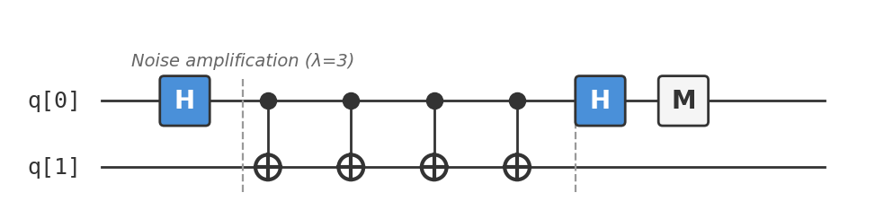
Scale 3: Noise-amplified circuit

Insert two CNOT pairs (each pair is logically identity but adds gate noise):

h q[0];
cx q[0], q[1]; cx q[0], q[1];   // pair 1: CX·CX = I
cx q[0], q[1]; cx q[0], q[1];   // pair 2: CX·CX = I
h q[0];
measure q[0] -> c[0];

Logically identical to Scale 1, but with 4 extra CNOTs worth of noise. The noise is approximately 3× the original (1 base + 4 identity gates ≈ 3× noise).

Scale 5: More noise

Insert four CNOT pairs (8 extra CNOTs):

h q[0];
cx q[0], q[1]; cx q[0], q[1];   // pair 1
cx q[0], q[1]; cx q[0], q[1];   // pair 2
cx q[0], q[1]; cx q[0], q[1];   // pair 3
cx q[0], q[1]; cx q[0], q[1];   // pair 4
h q[0];
measure q[0] -> c[0];

Approximately 5× noise.

Extrapolation

With three data points \((\lambda_1, E_1), (\lambda_3, E_3), (\lambda_5, E_5)\), extrapolate to \(\lambda = 0\):

Linear (2 points):

\[E_0 \approx E_1 - \frac{E_3 - E_1}{3 - 1} \times 1 = \frac{3E_1 - E_3}{2}\]

Richardson (3 points):

\[E_0 \approx \frac{15E_1 - 10E_3 + 3E_5}{8}\]

The complete circuits

Three QASM files, one per noise scale:

• zne_scale1.qasm — base circuit (\(\lambda = 1\))
• zne_scale3.qasm — 3× noise (\(\lambda = 3\))
• zne_scale5.qasm — 5× noise (\(\lambda = 5\))

Run it

Run all three circuits on your Quokka. On a perfect simulator, all three give \(|0\rangle\) every time (\(\langle X \rangle = 1.0\)). The technique only shows its value on noisy hardware.

Example noisy results (1% depolarizing error per CNOT):

Scale \(\lambda\)	Counts	\(\langle X \rangle\)
1	\(\{0: 966, 1: 58\}\)	\(0.89\)
3	\(\{0: 921, 1: 103\}\)	\(0.80\)
5	\(\{0: 871, 1: 153\}\)	\(0.70\)

Linear extrapolation (\(\lambda = 1, 3\)): \(E_0 \approx \frac{3 \times 0.89 - 0.80}{2} = 0.94\)

Richardson extrapolation (\(\lambda = 1, 3, 5\)): \(E_0 \approx \frac{15 \times 0.89 - 10 \times 0.80 + 3 \times 0.70}{8} = 0.93\)

Both are closer to the ideal (\(1.0\)) than the raw \(0.89\). Not perfect — but you got a better answer without any hardware improvements.

Apply this to any circuit note

ZNE works on any circuit. To mitigate Circuit Bench 01 (Bell State), for example, replace the CNOT with three CNOTs (CX·CX·CX = CX) for \(\lambda = 3\), and five for \(\lambda = 5\). Then extrapolate the correlation measurement.

Extend and experiment

1. Separate logic from noise. Run all three files on an ideal simulator first: each should return 0 every time. Then run the same files on noisy hardware. Only the noisy results should form a decay trend; if the ideal outputs differ, the scaled circuits are not logically equivalent.
2. Add a fourth noise scale. Copy zne_scale5.qasm and add two more CNOT pairs, giving six pairs in total for a nominal \(\lambda=7\) point. Refit with and without the new point. A longer fit is useful only while a measurable signal remains.
3. Break an identity pair deliberately. Remove one CNOT from a pair and run on an ideal simulator. The output changes because the circuit logic has changed, so extrapolating that point would be invalid. This negative control tests the central ZNE assumption rather than the fitting formula.

Analysis

The noise model: depolarizing channels

ZNE assumes noise increases smoothly with the number of gates. The simplest model: each gate applies a depolarizing channel with probability \(p\):

\[\mathcal{E}(\rho) = (1 - p)\rho + \frac{p}{d}I\]

where \(d\) is the Hilbert space dimension. This replaces the state with the maximally mixed state with probability \(p\).

After \(n\) gates, the expectation value decays as:

\[E_n = (1 - p)^n E_{\text{ideal}}\]

This is an exponential decay in \(n\). If noise scaling increases \(n\) by factor \(\lambda\):

\[E(\lambda) = (1 - p)^{\lambda n} E_{\text{ideal}} = e^{-\lambda n \ln(1/(1-p))} E_{\text{ideal}}\]

Extrapolating \(E(\lambda)\) to \(\lambda = 0\) gives \(E_{\text{ideal}}\) exactly if the exponential model is correct. In practice, the model is approximate, so the extrapolation improves but doesn't perfect the result.

Richardson extrapolation: the math

Given \(m\) data points at noise scales \(\lambda_1 < \lambda_2 < \cdots < \lambda_m\), Richardson extrapolation fits a polynomial of degree \(m - 1\) through the points and evaluates at \(\lambda = 0\).

The zero-noise estimate is:

\[E_0 = \sum_{k=1}^{m} \gamma_k E(\lambda_k)\]

where the coefficients \(\gamma_k\) satisfy:

\[\sum_{k=1}^{m} \gamma_k = 1 \quad \text{and} \quad \sum_{k=1}^{m} \gamma_k \lambda_k^j = 0 \quad \text{for } j = 1, \ldots, m-1\]

For 2 points (\(\lambda = 1, 3\)): \(\gamma_1 = 3/2\), \(\gamma_2 = -1/2\):

\[E_0 = \frac{3E_1 - E_3}{2}\]

For 3 points (\(\lambda = 1, 3, 5\)): \(\gamma_1 = 15/8\), \(\gamma_2 = -10/8\), \(\gamma_3 = 3/8\):

\[E_0 = \frac{15E_1 - 10E_3 + 3E_5}{8}\]

Higher-order extrapolation cancels higher-order noise terms but amplifies statistical fluctuations. In practice, 2–3 points is optimal for most hardware noise levels.

Other error mitigation techniques

ZNE is just one technique. The error mitigation zoo includes:

Technique	Idea	Overhead	Limitations
ZNE	Extrapolate to zero noise	2–5× circuit runs	Assumes smooth noise scaling
Probabilistic error cancellation (PEC)	Quasi-probability decomposition of ideal gates	Exponential in circuit depth (\(\gamma^{2d}\) samples)	Requires noise characterization
Clifford data regression (CDR)	Learn error model from near-Clifford circuits	Moderate	Assumes simple noise
Symmetry verification	Post-select on known symmetries	Discards some shots	Needs problem-specific symmetries
Twirling	Convert coherent errors to stochastic	Negligible	Doesn't reduce stochastic noise
Classical shadows	Efficient observable estimation	Many circuits	Statistical technique, not mitigation

PEC is the gold standard — it gives an unbiased estimate of the noiseless result — but the sample overhead grows exponentially with circuit depth. ZNE offers a practical middle ground: moderate improvement with modest overhead.

When does ZNE fail?

ZNE works well when:

• Noise scales linearly with the number of gates
• The noise is roughly gate-independent (each gate adds similar noise)
• The circuit is short enough that the signal hasn't completely decayed

ZNE breaks down when:

• Non-Markovian noise: Noise that depends on the history of operations (crosstalk, drift)
• Measurement errors: ZNE as described only mitigates gate noise. Measurement errors need separate calibration
• Signal near zero: If the noisy expectation is already close to 0 (fully depolarized), extrapolation amplifies noise more than signal
• Very deep circuits: The exponential decay means there's simply no signal left to extrapolate

For practical VQE-style circuits (tens to low hundreds of gates), ZNE typically improves results by 10–50%.

Practical notes

• This is the most practical Circuit Bench note. Most other notes assume near-perfect execution. This one deals with reality. If you're running on real hardware, ZNE is your first line of defense.

• The circuits are intentionally simple. We use a 1-qubit circuit to illustrate the concept clearly. On a real problem, you'd apply ZNE to your actual algorithm circuit (Grover, VQE, QAOA) by inserting identity-gate pairs around the critical gates.

• On a simulator, all three circuits give the same result. ZNE is invisible on a perfect simulator. You need actual hardware noise (or a noise model) to see the benefit.

• If you liked this, try: Circuit Bench 12 (Quantum Counting) is the final note in this sequence. It combines Grover's search (Circuit Bench 06) with QPE (Circuit Bench 10) — two powerful algorithms working together.