Circuit Bench 08: VQE for H2

This note shows the circuit-level core of a Variational Quantum Eigensolver (VQE) calculation for a reduced two-qubit model of the hydrogen molecule.

It is not a full chemistry pipeline. The molecular Hamiltonian has already been reduced to qubit operators, and the circuit below is one trial state in the variational loop. The goal is to make the moving parts visible: state preparation, a parameterised ansatz, basis changes, measurement, and energy reconstruction.

What this circuit does

VQE tries to estimate the ground-state energy of a Hamiltonian \(H\). For a trial state \(|\psi(\theta)\rangle\), the variational principle says

\[ \langle \psi(\theta) | H | \psi(\theta) \rangle \geq E_0, \]

where \(E_0\) is the true ground-state energy. A classical optimiser changes \(\theta\); the quantum device prepares the state and measures the terms needed to estimate the energy.

For the reduced H2 model used in the companion notebook, the Hamiltonian has the form

\[ H = g_0 I + g_1 Z_0 + g_2 Z_1 + g_3 Z_0 Z_1 + g_4 X_0 X_1 + g_5 Y_0 Y_1 . \]

That means one circuit run is not enough. The \(Z\) terms, \(X_0X_1\) term, and \(Y_0Y_1\) term are estimated with different measurement bases and then combined with the coefficients.

Files on the bench

Open the source directory on GitHub.

File	Purpose
vqe_h2_zz.qasm	Prepare one trial state and measure its Z-basis terms
expected.txt	Expected occupation patterns and measurement limits
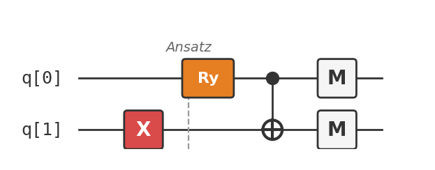
circuit.png	Trial-state circuit diagram

Circuit walkthrough

The public QASM file, vqe_h2_zz.qasm, shows the \(Z\)-basis measurement circuit for one trial angle.

OPENQASM 2.0;
include "qelib1.inc";

qreg q[2];
creg c[2];

// Hartree-Fock reference state for this qubit ordering
x q[1];

// One trial point in the variational ansatz
ry(1.570796) q[0];
cx q[0], q[1];

// Z-basis measurement
measure q[0] -> c[0];
measure q[1] -> c[1];

The first line after the registers prepares the reference occupation pattern used by the reduced model. The ry rotation introduces the variational parameter. The cx entangles the two qubits so the trial state can mix two occupation patterns rather than staying a single classical bit string.

For a full energy estimate, run related circuits with basis rotations before measurement:

Term	Basis rotation before measurement	What the counts estimate
\(Z_0\), \(Z_1\), \(Z_0Z_1\)	none	occupation-basis expectations
\(X_0X_1\)	h on both qubits	correlation in the \(X\) basis
\(Y_0Y_1\)	sdg then h on both qubits	correlation in the \(Y\) basis

This is why VQE is a measurement workflow, not just a single pretty circuit diagram.

Run it

Run vqe_h2_zz.qasm on a simulator or compatible OpenQASM 2.0 runner. In the displayed q[0] q[1] order, the trial angle in this file should put most of the probability on the two occupation patterns 01 and 10.

For 1024 ideal shots, a typical result is approximately:

{'01': 512, '10': 512}

Shot noise will move the counts around. The important feature is that the circuit is no longer a single Hartree-Fock bit string; the ansatz has created a superposition that can be tested in several measurement bases.

Extend and experiment

1. Sweep the ansatz angle. Replace ry(1.570796) with 0, \(\pi/2\), and \(\pi\). In displayed q[0] q[1] order, the ideal Z-basis result moves from 01, through an equal 01/10 mixture, to 10. This exposes how the parameter moves weight between the two occupation patterns.
2. Remove the entangler. Delete the CNOT while keeping the \(\pi/2\) rotation. The outcomes become 01 and 11 instead of 01 and 10: the second qubit remains fixed, so the ansatz is a product state rather than a correlated trial state.
3. Build the other measurement circuits. Make two copies of the file. For \(X_0X_1\), insert h on both qubits before measurement. For \(Y_0Y_1\), insert sdg followed by h on both. Those counts estimate different Pauli correlations; they are not a complete energy until a classical calculation combines them with the Hamiltonian coefficients.

What this shows

This small circuit shows the core VQE mechanics:

• a molecule becomes a qubit Hamiltonian;
• a parameterised circuit prepares a trial state;
• basis rotations turn different Pauli terms into measurable \(Z\)-basis counts;
• the measured expectations are combined into an energy;
• a classical optimiser repeats the process for new angles.

It also shows why VQE felt plausible for early hardware: the circuit can be shallow, while the expensive search is shared with a classical optimiser.

What this does not show

This is not a scalable drug-discovery calculation. It does not generate molecular integrals, choose an active space, scan bond lengths, or optimise a production ansatz. It also does not remove the measurement problem: larger molecular Hamiltonians can contain many Pauli terms, and each term needs enough shots to be useful.

Treat this as the smallest bench-top version of the idea. The companion Bottleneck notebook uses the same structure to sweep a parameter and compare the measured energy against exact diagonalisation of the reduced model.