The Eigensolver Zoo

Every eigensolver is a way of applying a function of the operator and letting the spectrum sort itself out. This post surveys the classical half: the methods that stretch.

Part 3 of Linear Algebra for Fun and Profit

Part 1 builds the spectral theorem. Part 2, Where Eigenvalues Pay Rent, shows why eigenvalues matter (PageRank, portfolio risk, molecular energy). This post surveys the classical tools; Part 4 crosses to quantum.

The eigenproblem and the spectral theorem

The eigenvalue problem is a request: given a linear operator \(H\), find the numbers \(E\) and nonzero vectors \(\ket{\psi}\) for which

\[H\ket{\psi} = E\ket{\psi}.\]

The number \(E\) is an eigenvalue and \(\ket{\psi}\) its eigenvector. We restrict to the case that matters here, \(H\) Hermitian (\(H = H^\dagger\)), because the operators of quantum mechanics are Hermitian and because that hypothesis is exactly what makes the problem well-behaved. The spectral theorem guarantees a complete orthonormal eigenbasis \(\{\ket{n}\}\) with real eigenvalues \(E_n\) and

\[H = \sum_n E_n \ket{n}\bra{n}.\]

Solving the eigenproblem means finding this decomposition, or the part of it one cares about. An eigensolver is any procedure that approximates some of the pairs \((E_n, \ket{n})\), most often the lowest one.

The ground state. Order the eigenvalues \(E_0 \le E_1 \le \cdots\). The lowest eigenvalue \(E_0\) is the ground energy and its eigenvector \(\ket{E_0}\) the ground state. The names are from physics, where \(H\) is an energy and the lowest-energy configuration is the one a cold system settles into. Most of this post concerns one narrowed request: find \(E_0\) and \(\ket{E_0}\).

Running example A: an abstract two-level system. Consider

\[H = \begin{pmatrix} 2 & 1 \\ 1 & 2 \end{pmatrix}, \qquad \ket{+} = \tfrac{1}{\sqrt2}\begin{pmatrix}1\\1\end{pmatrix}, \quad \ket{-} = \tfrac{1}{\sqrt2}\begin{pmatrix}1\\-1\end{pmatrix},\]

whose eigenvectors are \(\ket{+}\) and \(\ket{-}\) with eigenvalues \(3\) and \(1\). The ground state is \(\ket{-}\) with \(E_0 = 1\), not \(\ket{+}\); the ground state is the lowest, and \(1 < 3\). This example is small enough that every method can be checked by hand.

Running example B: the antiferromagnetic Heisenberg interaction. The physical example carried throughout is the two-spin Heisenberg interaction, a standard, exactly solvable model of two coupled spin-\(\tfrac12\) particles, built from the Pauli matrices \(X, Y, Z\):

\[H_{\mathrm{Heis}} = XX + YY + ZZ \equiv X\otimes X + Y\otimes Y + Z\otimes Z.\]

It is exactly solvable through one identity, \(XX + YY + ZZ = 2\,\mathrm{SWAP} - I\), where SWAP exchanges the two spins, \(\mathrm{SWAP}\ket{ab} = \ket{ba}\). SWAP has eigenvalue \(+1\) on states symmetric under exchange and \(-1\) on antisymmetric states, so

\[H_{\mathrm{Heis}} = \begin{cases} +1 & \text{on the symmetric triplet (three states),} \\ -3 & \text{on the antisymmetric singlet } \ket{s} = \tfrac{1}{\sqrt2}(\ket{01} - \ket{10}). \end{cases}\]

The ground state is the singlet with \(E_0 = -3\); the excited level is the triplet at \(+1\), threefold degenerate. "Antiferromagnetic" means the coupling favours the singlet, with anti-aligned spins. Example B reappears as the natural test case for the quantum methods in Part 4.

Functions of an operator

One identity underlies every method below. For a Hermitian \(H = \sum_n E_n \ket{n}\bra{n}\) and any function \(f\) given by a power series, \(f\) acts eigenvalue by eigenvalue:

\[f(H) = \sum_n f(E_n)\,\ket{n}\bra{n}.\]

In particular \(H^k = \sum_n E_n^{\,k}\ket{n}\bra{n}\), the propagator is \(e^{-iHt} = \sum_n e^{-iE_n t}\ket{n}\bra{n}\), and the stretch operators are \(e^{\pm Ht} = \sum_n e^{\pm E_n t}\ket{n}\bra{n}\). Every eigensolver in this post is one choice of \(f\), applied one way. Part 1 derives this identity from the matrix exponential; here it is simply the tool.

The variational principle and the Rayleigh quotient

Finding \(E_0\) looks like a search over an entire vector space. The variational principle turns it into a minimisation. A method is variational when it approximates the answer by optimising a quantity over a family of trial states. The quantity is the Rayleigh quotient of a nonzero trial vector \(\ket{\psi}\),

\[R(\psi) = \frac{\langle \psi \lvert H \rvert \psi \rangle}{\langle \psi | \psi \rangle}.\]

Expand \(\ket{\psi} = \sum_n c_n \ket{n}\) in the eigenbasis. Using \(H\ket{n} = E_n\ket{n}\) and orthonormality,

\[R(\psi) = \frac{\sum_n |c_n|^2 E_n}{\sum_n |c_n|^2}.\]

This is a weighted average of the eigenvalues, with weights \(|c_n|^2 \ge 0\). A weighted average can be no smaller than the smallest of the numbers and no larger than the largest, so

\[E_0 \;\le\; R(\psi) \;\le\; E_{\max} \quad\text{for every }\ket{\psi},\]

with equality on the left exactly when all the weight sits on the ground state. This is the variational principle,

\[E_0 = \min_{\psi \ne 0} R(\psi),\]

an exact, proven statement, not a heuristic. Its practical half is the one we use constantly: any trial state gives an upper bound on the ground energy, \(E_0 \le R(\psi)\), and a lower \(R\) means a better state. Minimising the Rayleigh quotient is therefore a way to search for the ground state, and it is the engine behind several methods below, from Rayleigh-quotient iteration to the variational quantum eigensolver in Part 4.

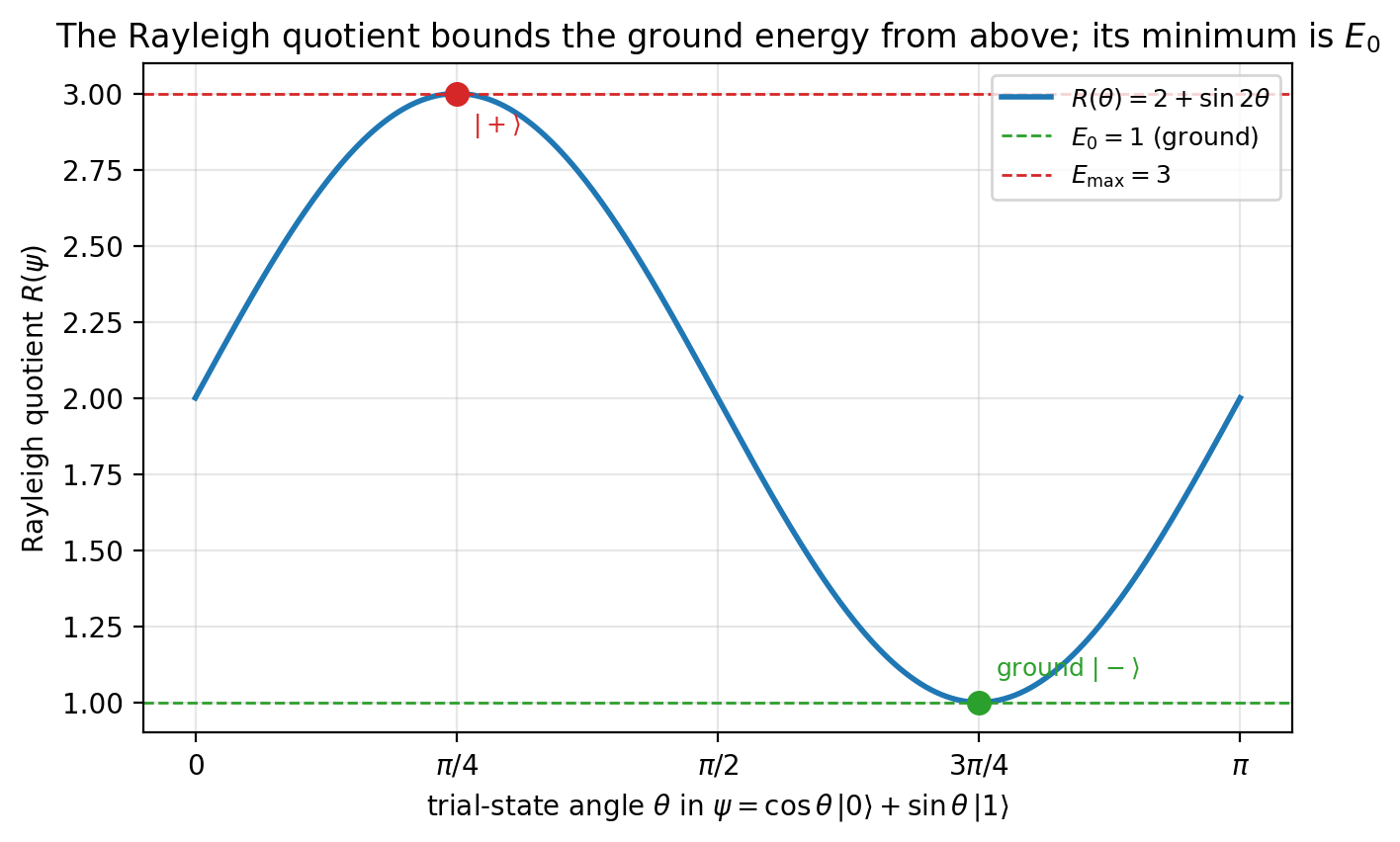
On example A. Try the site state \(\lvert 0\rangle = (1,0)^T\): \(R(\lvert 0\rangle) = \langle 0 \lvert H \rvert 0 \rangle = H_{00} = 2\), an upper bound on \(E_0 = 1\). Try \(\lvert -\rangle\): \(R(\lvert -\rangle) = 1 = E_0\), the exact minimum. Sweeping the real trial states \(\lvert\psi(\theta)\rangle = \cos\theta\,\lvert 0\rangle + \sin\theta\,\lvert 1\rangle\) gives the closed form \(R(\theta) = 2 + \sin 2\theta\): its minimum \(1\) at \(\theta = 3\pi/4\) is the ground state \(\lvert -\rangle\), and its maximum \(3\) at \(\theta = \pi/4\) is \(\lvert +\rangle\).

Why the ground state, and why the dimension makes it hard

Why the lowest eigenvalue. The ground-state problem is central across three settings. In physics, \(E_0\) is the energy of matter at zero temperature and \(\ket{E_0}\) encodes its phase (magnet, superconductor, spin liquid). In optimisation, a combinatorial problem (MaxCut, XORSAT, any Ising model) is encoded so that a classical cost is the energy of a diagonal Hamiltonian; the lowest-energy state is the optimal assignment, so "ground state" and "optimal solution" coincide. In numerical linear algebra and machine learning, extremal eigenpairs are the content of principal component analysis, spectral clustering, and graph methods, as Part 2 demonstrated.

Why it is hard. For a system of \(N\) two-level parts (spins, or sites), the state space is \(\mathbb{C}^{2^N}\) and \(H\) is a \(2^N \times 2^N\) matrix. Dense diagonalisation costs on the order of \((2^N)^3\) operations and \((2^N)^2\) memory, both exponential in \(N\). At \(N = 20\) the dimension is about \(10^6\); at \(N = 50\) the matrix cannot be stored, let alone factored.

What rescues it: structure. Physical Hamiltonians are sparse and local: \(H\) is a sum of a polynomial number of terms, each acting on only a few sites, so the matrix-vector product \(H\ket{v}\) can be computed without ever forming the dense matrix. Every method in the next section needs only this product. That is the dividing line: exact dense methods are exponential and general, while iterative methods are cheap but return only part of the spectrum, typically the extremes. The state vector itself still has \(2^N\) entries, and that memory wall, near \(N \approx 50\) on a single classical node, is what later motivates the quantum methods.

Classical eigensolvers

The workhorse classical eigensolvers share one feature: they need only the matrix-vector product \(H\ket{v}\), never the dense matrix, so they run wherever that product is cheap. They differ in which function of \(H\) they effectively apply.

Power iteration: the discrete stretch

The simplest method makes the spectrum sort itself. Start from a generic vector and apply \(H\) repeatedly:

\[\ket{v_0} = \sum_n c_n \ket{n} \;\Longrightarrow\; H^k \ket{v_0} = \sum_n c_n E_n^{\,k} \ket{n}.\]

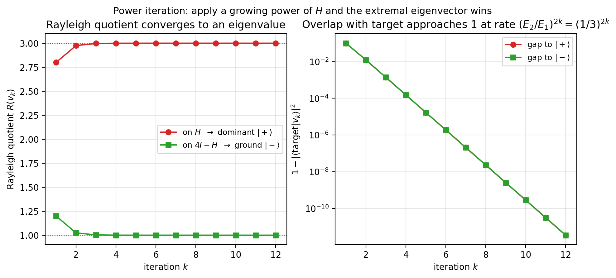
The component with the largest \(|E_n|\) is multiplied by the largest factor at each step, so after normalising, \(H^k\ket{v_0} / \lVert H^k\ket{v_0}\rVert\) tends to the eigenvector of largest-magnitude eigenvalue, the dominant eigenvector. The error shrinks geometrically at the rate \(|E_2/E_1|^k\).

This is the discrete form of the stretch operator. Written through the spectral decomposition, \(e^{+Ht} = \sum_n e^{E_n t}\ket{n}\bra{n}\) stretches each eigendirection by \(e^{E_n t}\), so the largest eigenvalue runs away with the vector as \(t\) grows. Power iteration is the same idea in discrete steps: apply a growing function of \(H\) and the extremal eigenvector wins. The imaginary-time method below is the continuous version aimed at the ground state.

Targeting the ground state by a shift. Plain power iteration finds the dominant eigenvalue, not usually the lowest. A shift fixes this: applying \((\sigma I - H)\) gives eigenvalues \(\sigma - E_n\), and for a \(\sigma\) that makes \(\sigma - E_0\) the largest in magnitude, the ground state becomes dominant. On example A, \(H\) has eigenvalues \(\{1, 3\}\), so plain power iteration converges to \(\ket{+}\) (\(E = 3\)). Iterating instead on \(4I - H\), whose eigenvalues \(\{3, 1\}\) attach to \(\{\ket{-}, \ket{+}\}\), makes the ground state dominant, and the iteration converges to it with \(R(v_k) \to E_0 = 1\).

The same three lines that rank the web

Power iteration is not only for Hamiltonians. Ask a different question, "who matters in a network?", and the same machinery answers it. Declare a node important when important nodes link to it, \(x_i \propto \sum_j A_{ij} x_j\), where \(A\) is the adjacency matrix. That circular definition is an eigenvector equation, \(Ax = \lambda x\), and the sensible scores are the dominant eigenvector, all-positive by the Perron-Frobenius theorem. To compute it, start everyone equal and repeatedly replace each score by the sum of its neighbours' scores: the power iteration just described, applied to \(A\).

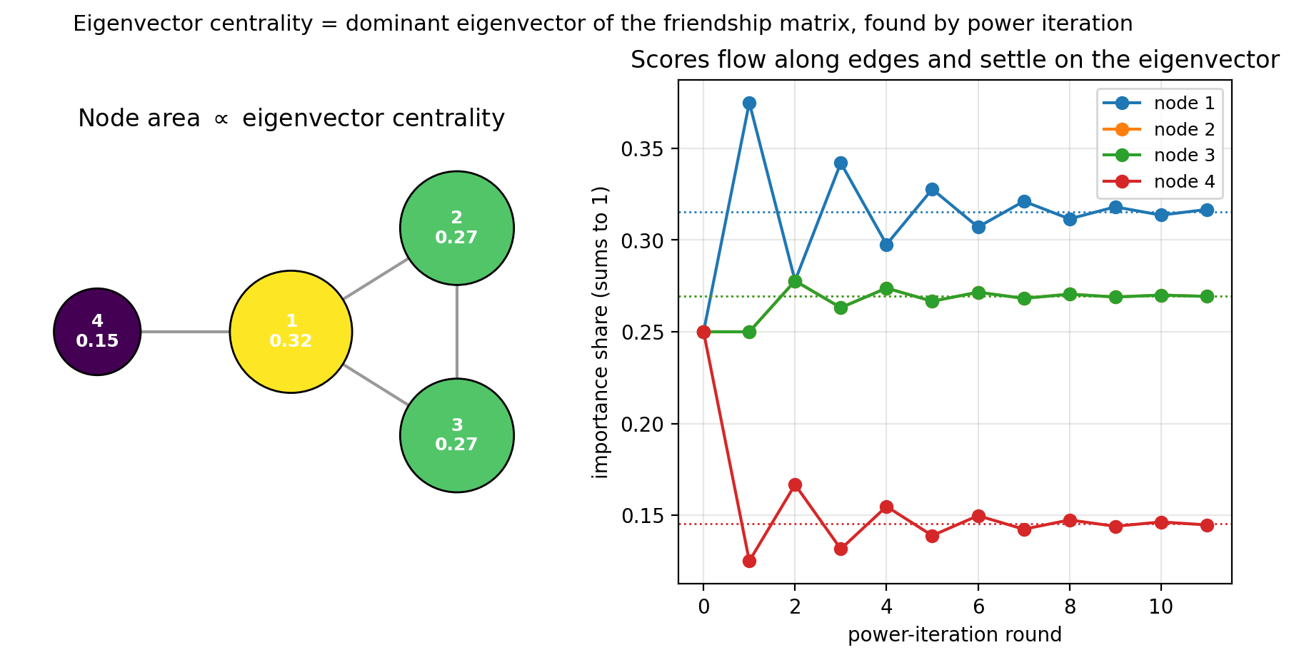
On the four-node network shown (node 1 a hub; 2 and 3 also linked; 4 a leaf), the scores flow from a flat start onto the eigenvector \((0.315, 0.270, 0.270, 0.145)\) in a handful of rounds. Node 4 sits beside the hub yet ranks last, because importance must flow both ways to accumulate; nodes 2 and 3 stay identical, as their symmetry demands. This is exactly Google's original PageRank³: the dominant eigenvector of the web's link matrix, found by power iteration. Recommendation systems are the same idea on a ratings matrix⁴: its leading singular vectors, the eigenvectors of \(R^\top R\), are the latent "taste axes" (this is principal component analysis). Whether the operator is a Hamiltonian, a friendship graph, or a ratings matrix, the question is the same, "which eigenvector?", and so is the tool, "apply a function of the operator and let the extremal direction win."

Inverse and shifted iteration

Power iteration converges only as fast as the eigenvalue gap allows, and it targets the dominant eigenvalue. Inverse iteration targets any eigenvalue by iterating with \((H - \sigma I)^{-1}\), whose eigenvalues \(1/(E_n - \sigma)\) are largest for the \(E_n\) closest to the shift \(\sigma\). Choosing \(\sigma\) just below the spectrum drives the iteration to the ground state. Rayleigh-quotient iteration updates the shift to the current Rayleigh quotient at every step, \(\sigma_k = R(v_k)\), which for Hermitian \(H\) converges cubically once close. The price is that each step solves a linear system \((H - \sigma I)\ket{x} = \ket{v}\) rather than doing a single product.

Krylov subspace methods and Lanczos

Power iteration keeps only the last vector \(H^k\ket{v}\) and discards the intermediates. That is wasteful: the sequence \(\ket{v}, H\ket{v}, H^2\ket{v}, \dots\) spans the Krylov subspace

\[\mathcal{K}_m = \operatorname{span}\{\ket{v}, H\ket{v}, \dots, H^{m-1}\ket{v}\},\]

and the best eigenvalue estimates within it are far better than the last iterate alone. Restricting \(H\) to \(\mathcal{K}_m\) and diagonalising the small restriction, the Rayleigh-Ritz procedure, yields the Ritz values that approximate the extremal eigenvalues of \(H\).

For Hermitian \(H\), the Lanczos algorithm¹ builds an orthonormal basis of \(\mathcal{K}_m\) in which \(H\) is tridiagonal, so the Ritz values are the eigenvalues of a small tridiagonal matrix. A handful of matrix-vector products then gives the ground energy to high accuracy; convergence to the extremes is governed by Chebyshev polynomials and is much faster than the plain eigenvalue-ratio rate of power iteration. In these terms, a Krylov method applies the best polynomial in \(H\) of a given degree rather than the fixed monomial \(H^k\). Lanczos is the classical state of the art for extremal eigenpairs of large sparse Hermitian matrices², and it is the honest baseline against which any quantum eigensolver must be judged.

The wall that motivates quantum methods. Every method here stores the state vector, \(2^N\) complex numbers, and applies \(H\) to it classically. When \(2^N\) exceeds classical memory, near \(N \approx 50\) on a single node, even a matrix-free Lanczos step cannot be taken. The quantum eigensolvers of Part 4 represent the same \(2^N\)-dimensional state in \(N\) physical qubits, trading the memory wall for the difficulty of preparing and measuring quantum states.

Imaginary time: the ground-seeking stretch

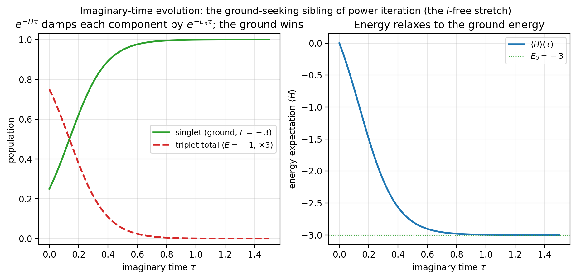
Replace the real time \(t\) by \(-i\tau\) in the propagator. The rotation becomes a stretch,

\[e^{-H\tau} = \sum_n e^{-E_n\tau}\ket{n}\bra{n},\]

the same stretch operator with a real exponent. Each eigencomponent is damped by \(e^{-E_n\tau}\), so the lowest eigenvalue is damped the least and, after renormalising, takes over:

\[\lvert\psi(\tau)\rangle = \frac{e^{-H\tau}\lvert\psi_0\rangle}{\lVert e^{-H\tau}\lvert\psi_0\rangle\rVert} \;\xrightarrow[\ \tau\to\infty\ ]{}\; \lvert E_0\rangle, \qquad \text{provided } \langle E_0 | \psi_0 \rangle \ne 0.\]

This is power iteration again, now continuous and aimed at the ground state: where power iteration applied a growing power \(H^k\) to reach the dominant eigenvector, imaginary time applies a growing exponential \(e^{-H\tau}\) to reach the lowest. The two are one idea, the \(i\)-free stretch, discrete and continuous.

The catch. \(e^{-H\tau}\) is not unitary, so a quantum computer cannot apply it directly; unitary hardware performs rotations, not stretches. Quantum imaginary-time evolution approximates each non-unitary step by a fitted sequence of unitaries; other routes use block encodings, engineered dissipation, or measurement. Imaginary time is the cleanest ground-state filter in principle, but realising a non-unitary map on unitary hardware is the difficulty.

The landscape so far

Every method in this post is a function of \(H\) with a real exponent: a stretch. Power iteration uses \(H^k\), imaginary time uses \(e^{-H\tau}\), Lanczos uses the best polynomial. They all amplify the extremal eigenvector. The stretch side of the landscape:

method	function of \(H\)	effect
dense diagonalisation	all of \(H\) at once	exact, exponential cost
power iteration	\(H^k\) (stretch)	to the dominant eigenvector
shifted / inverse iteration	\((\sigma I - H)^k\) or \((H - \sigma I)^{-1}\)	to a targeted eigenvector
Lanczos	best polynomial in \(H\) on the Krylov subspace	to the extremes, fast
imaginary time	\(e^{-H\tau}\) (stretch)	to the ground state

Part 4 introduces the quantum methods, where the exponent gains a factor of \(i\) and stretch becomes rotation.

---

1. C. Lanczos, "An iteration method for the solution of the eigenvalue problem of linear differential and integral operators," J. Res. Natl. Bur. Stand. 45, 255–282 (1950). ↩

2. G. H. Golub and C. F. Van Loan, Matrix Computations, 4th ed., Johns Hopkins University Press (2013). ↩

3. L. Page, S. Brin, R. Motwani, and T. Winograd, "The PageRank Citation Ranking: Bringing Order to the Web," Stanford InfoLab Technical Report (1999). ↩

4. Y. Koren, R. Bell, and C. Volinsky, "Matrix Factorization Techniques for Recommender Systems," IEEE Computer 42(8), 30–37 (2009). ↩