What a Difference i Makes

The classical eigensolvers of Part 3 stretch. Insert a factor of \(i\) into the exponent and stretching becomes rotation: the eigenvalues move onto the unit circle, lengths are preserved, and a quantum computer can run the evolution natively. That single letter is the entire difference.

Part 4 of Linear Algebra for Fun and Profit

Part 1 builds the spectral theorem. Part 2 shows where eigenvalues pay rent. Part 3 surveys the classical eigensolvers (the stretch). This post crosses to the quantum side (the rotation).

From stretch to rotation

Part 3's methods all applied functions of \(H\) with real exponents, \(H^k\), \(e^{-H\tau}\), which stretch the spectrum and amplify an extremal eigenvector. Every one of them stores the full \(2^N\)-dimensional state vector, and every one hits the memory wall near \(N \approx 50\). A quantum computer represents that state in \(N\) qubits, each a physically realised two-level system, but its native operation is unitary evolution, rotation, not stretch. The tool is the propagator \(e^{-iHt}\), and the \(i\) is what makes it unitary.

Real-time evolution and quantum phase estimation

A quantum computer's native operation is real-time evolution: for local \(H\) it can apply the propagator \(e^{-iHt}\), the unitary that advances a quantum state by time \(t\), in polynomial depth. Through the spectral decomposition, \(e^{-iHt} = \sum_n e^{-iE_n t}\ket{n}\bra{n}\), so an eigenstate merely collects a unit-modulus factor, its eigenphase:

\[e^{-iHt}\ket{n} = e^{-iE_n t}\ket{n}.\]

Quantum phase estimation (QPE)¹² is the circuit that reads that eigenphase, and hence the eigenvalue \(E_n\), out of the state.

The mechanism. An ancilla register of \(m\) qubits — extra qubits used only to read out the phase — is placed in uniform superposition and used to apply controlled evolutions \(e^{-iH\,2^j t_0}\) for \(j = 0, 1, \dots, m-1\). Acting on an eigenstate \(\ket{n}\), these imprint the phase \(E_n\) across the register in binary; an inverse quantum Fourier transform turns that imprinted phase into a number, read off by measuring the ancillas.

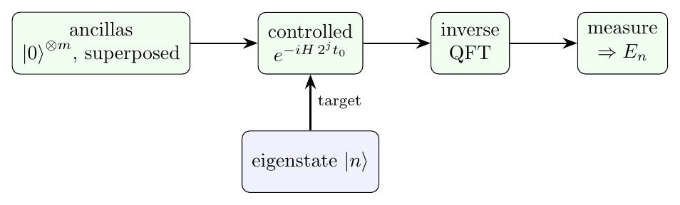
Precision and cost. With \(m\) ancilla bits the phase is resolved to about \(2^{-m}\), and the total evolution time scales as \(1/\varepsilon\) for precision \(\varepsilon\). This Heisenberg-limited scaling — the best precision-per-unit-evolution-time any quantum strategy allows — is quadratically better in time than estimating an energy by averaging measurements. That is the ideal statement: QPE needs long, coherent, controlled evolution and an inverse Fourier transform, which places it in the fault-tolerant era. It is not a near-term method.

The input problem. QPE needs an eigenstate to read. Fed a general state \(\ket{\psi} = \sum_n c_n \ket{n}\), it returns the eigenvalue \(E_n\) with probability \(|c_n|^2\), projecting the state onto \(\ket{n}\) as it does so. To obtain the ground energy one therefore needs a trial state with appreciable overlap \(|c_0|^2\) with the ground state, which is itself the state-preparation problem the other methods address.

The rotation branch. QPE is the rotation side of the one idea: it uses \(e^{-iHt}\), the length-preserving rotation, purely to read eigenphases, whereas the stretch methods of Part 3 drive a state toward an eigenvector. On example A, \(e^{-iHt}\) has eigenphases \(e^{-3it}\) and \(e^{-it}\); supplied the ground state \(\ket{-}\) it returns \(E_0 = 1\), and supplied \(\ket{0} = \tfrac{1}{\sqrt2}(\ket{+} + \ket{-})\) it returns \(3\) or \(1\), each with probability \(\tfrac12\). On example B, supplied the singlet it returns \(E_0 = -3\).

Adiabatic preparation: the unitary cousin

Adiabatic preparation³ reaches the ground state while staying unitary. Begin in the easily prepared ground state of a simple \(H_0\), and interpolate slowly,

\[H(s) = (1-s)\,H_0 + s\,H_1, \qquad s: 0 \to 1.\]

The adiabatic theorem states that if the interpolation is slow compared with the inverse square of the smallest spectral gap \(\Delta_{\min}\) encountered, the system stays in the instantaneous ground state and ends in the ground state of \(H_1\). This is real-time evolution under a time-dependent Hamiltonian, so it is implementable on unitary hardware, at a runtime that scales as \(1/\Delta_{\min}^2\). The guarantee is proven under the gap condition, but hard problems tend to have small gaps, and the gap is the binding cost. The quantum approximate optimisation algorithm (QAOA)⁴, a discretised, tunable descendant of this annealing idea, is the thread picked up next.

The variational quantum eigensolver

The variational quantum eigensolver (VQE)⁵⁶ marries the variational principle with a quantum computer's ability to prepare and measure states. It is the near-term counterpart to QPE: shallow circuits and a classical loop in place of deep coherent evolution.

The loop. Choose a parameterised circuit, the ansatz, preparing \(\ket{\psi(\theta)} = U(\theta)\ket{\psi_0}\), then repeat:

1. on the quantum device, estimate the energy \(E(\theta) = \langle \psi(\theta) \lvert H \rvert \psi(\theta) \rangle\) by measuring each term of \(H = \sum_a c_a P_a\) and combining;
2. a classical optimiser proposes parameters \(\theta\) that lower \(E(\theta)\);
3. stop when the energy stops improving.

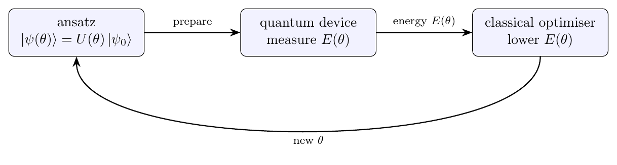
By the variational principle, every \(E(\theta)\) is an upper bound on \(E_0\), and the lowest one found is the estimate. VQE is thus "minimise the Rayleigh quotient over the manifold the ansatz can reach." On example A with the one-parameter ansatz \(\ket{\psi(\theta)} = \cos\theta\,\ket{0} + \sin\theta\,\ket{1}\), the landscape is exactly \(R(\theta) = 2 + \sin 2\theta\), minimised at the ground state \(\ket{-}\).

Why use a quantum computer. The state \(\ket{\psi(\theta)}\) lives in \(2^N\)-dimensional space but is stored in \(N\) qubits and prepared by a polynomial-size circuit, so VQE can reach trial states that are hard to write down classically, and for local \(H\) the energy is efficient to measure. Ansätze range from hardware-efficient layers of rotations and entanglers to physically motivated forms (unitary coupled cluster in chemistry; the Hamiltonian-variational or QAOA ansatz for combinatorial and spin problems). On example B, an ansatz able to reach the singlet finds \(E_0 = -3\); an ansatz confined to the symmetric subspace cannot leave the triplet and is stuck at \(+1\), a first glimpse of how symmetry can trap a variational search in the wrong sector.

Honest limitations. VQE provides a rigorous variational upper bound, which is proven; whether it reaches \(E_0\) is not guaranteed, and four issues bound it in practice.

• Measurement cost. Estimating \(E(\theta)\) to precision \(\varepsilon\) needs on the order of \(1/\varepsilon^2\) samples per term, and the many Pauli terms of \(H\) multiply this into a serious overhead.
• Barren plateaus. For many expressive or deep ansätze, gradients vanish exponentially in \(N\), so the landscape is exponentially flat and training does not scale⁷.
• Local minima. The optimisation is non-convex; the classical optimiser can settle in a local minimum above \(E_0\).
• Expressibility versus trainability. An ansatz too small to represent the ground state gives a loose bound, while making it more expressive tends to worsen the plateau problem; the two pull against each other.

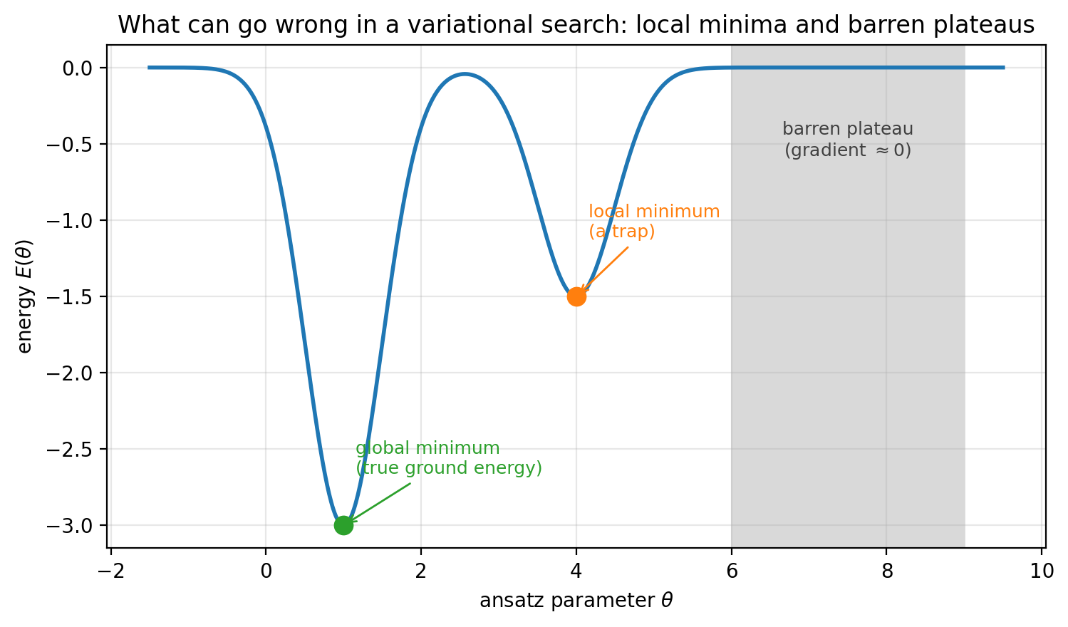
VQE is a heuristic with a rigorous bound but no general convergence or accuracy guarantee. Its trade against QPE is the era it suits: shallow circuits and a measurement-heavy classical loop, rather than deep coherent evolution with a precision guarantee.

Beyond per-instance optimisation

VQE and its structured relative QAOA share a defining cost: their parameters \(\theta\) are optimised per instance. Each new Hamiltonian restarts the classical loop and pays again the measurement overhead, the barren-plateau risk, and the local minima above. A natural question closes this post: is that per-instance optimisation always necessary?

There is empirical reason to think not. For several structured ansätze, good parameters are observed to concentrate⁸⁹: the values that work for one instance work, after a simple rescaling, for other instances of the same family, and often for larger sizes and greater depths. Where such regularity holds, the parameters can be set from a fitted schedule rather than optimised afresh, turning a variational method into a non-variational one. This trades per-instance optimisation for a one-time fit, at the risk that the regularity is only approximate. Parameter concentration is an empirical observation for particular families, not a theorem; whether it holds for a given problem, and how much accuracy is lost by setting rather than optimising, must be measured case by case. That measurement is an active research direction, and it is where a general introduction to eigensolvers hands off to specialised study.

The landscape as functions of \(H\)

Every method across Parts 3 and 4 is one choice of a function of \(H\) and one way of applying it. That is the single organising idea.

method	function of \(H\)	effect
dense diagonalisation	all of \(H\) at once	exact, exponential cost
power iteration	\(H^k\) (stretch)	to the dominant eigenvector
shifted / inverse iteration	\((\sigma I - H)^k\) or \((H - \sigma I)^{-1}\)	to a targeted eigenvector
Lanczos	best polynomial in \(H\) on the Krylov subspace	to the extremes, fast
imaginary time	\(e^{-H\tau}\) (stretch)	to the ground state
adiabatic	time-ordered \(e^{-i\int H(s)\,ds}\)	to the ground state, if slow versus the gap
phase estimation	\(e^{-iHt}\) (rotation)	reads an eigenphase \(E_n\)
VQE / QAOA	minimise \(R(\psi(\theta))\) over an ansatz	variational upper bound on \(E_0\)
set-parameter QAOA	ansatz with parameters set from a fitted schedule	non-variational, if parameters concentrate

The stretch operators, \(H^k\), \(e^{-H\tau}\), and the annealing limit, drive a state toward an extremal eigenvector; the rotation operator \(e^{-iHt}\) exposes eigenphases to be read; and the Rayleigh quotient turns the ground-state search into a minimisation. Classical methods apply these to a stored \(2^N\)-vector until the memory wall; quantum methods apply them to \(N\) qubits, trading that wall for the cost of coherent evolution, measurement, and state preparation.

The difference between the machine-learning half of all this and the quantum half is, as promised, a single factor of \(i\): real exponents stretch and rank (PageRank, principal component analysis, imaginary-time ground states), the imaginary exponent rotates and reads (phase estimation). Same spectral theorem, same functions of \(H\); one factor of \(i\) apart.

What this series built

Four posts, one idea. A Hermitian matrix has real eigenvalues on an orthonormal basis. Functions of the matrix act eigenvalue-by-eigenvalue. The real exponential stretches and the imaginary exponential rotates, and that single factor of \(i\) separates classical machine learning from quantum mechanics. The spectral theorem is not a textbook curiosity; it is the load-bearing structure under web search, portfolio risk, molecular simulation, and every eigensolver classical or quantum. That is the linear algebra. The fun was building it; the profit is what it computes.

---

1. A. Y. Kitaev, "Quantum measurements and the Abelian Stabilizer Problem," arXiv:quant-ph/9511026 (1995). ↩

2. M. A. Nielsen and I. L. Chuang, Quantum Computation and Quantum Information, Cambridge University Press (2010). ↩

3. E. Farhi, J. Goldstone, S. Gutmann, and M. Sipser, "Quantum Computation by Adiabatic Evolution," arXiv:quant-ph/0001106 (2000). ↩

4. E. Farhi, J. Goldstone, and S. Gutmann, "A Quantum Approximate Optimization Algorithm," arXiv:1411.4028 (2014). ↩

5. A. Peruzzo, J. McClean, P. Shadbolt, M.-H. Yung, X.-Q. Zhou, P. J. Love, A. Aspuru-Guzik, and J. L. O'Brien, "A variational eigenvalue solver on a quantum processor," Nat. Commun. 5, 4213 (2014); arXiv:1304.3061. ↩

6. J. R. McClean, J. Romero, R. Babbush, and A. Aspuru-Guzik, "The theory of variational hybrid quantum-classical algorithms," New J. Phys. 18, 023023 (2016); arXiv:1509.04279. ↩

7. J. R. McClean, S. Boixo, V. N. Smelyanskiy, R. Babbush, and H. Neven, "Barren plateaus in quantum neural network training landscapes," Nat. Commun. 9, 4812 (2018); arXiv:1803.11173. ↩

8. F. G. S. L. Brandão, M. Broughton, E. Farhi, S. Gutmann, and H. Neven, "For Fixed Control Parameters the Quantum Approximate Optimization Algorithm's Objective Function Value Concentrates for Typical Instances," arXiv:1812.04170 (2018). ↩

9. L. Zhou, S.-T. Wang, S. Choi, H. Pichler, and M. D. Lukin, "Quantum Approximate Optimization Algorithm: Performance, Mechanism, and Implementation on Near-Term Devices," Phys. Rev. X 10, 021067 (2020); arXiv:1812.01041. ↩